|
coupled chemistry-climate models |
  |
|
coupled chemistry-climate models |
|
| BACK |
Table of core processes for validating CCMs
with a focus on the model's ability to predict
future
ozone
Up-to-date
version of the CCMVal Evaluation Table available here.
|
Process-Oriented Validation of Coupled Chemistry-Climate Models |
| Overall Coordination Veronika Eyring, Neil Harris, and Ted Shepherd | |||||
| Process | Diagnostic* | Variables | Data | References | Contact |
| Dynamics Coordination: Martin Dameris and Paul Newman | |||||
| Forcing and propagation of planetary waves | Wave frequency analysis (WFA)
Planetary Wave (PW) spectrum (variances & co-variances) |
Temperature, Geopotential
Height, horizontal
winds
High-frequency (daily) data |
Met. Analyses ** | Mager and Dameris, 2004 | F.
Mager
M. Dameris |
| Hemispheric Ozone Variability Indices | Total column ozone over several years | Satellite data of total column ozone (e.g. TOMS, GOME) | Erbertseder et al., 2004 | T. Erbertseder | |
| Stratospheric response to wave drag | Annual cycle of temperatures in tropics and extra-tropics | Zonal monthly mean temperature, residual streamfunction | Met. Analyses
**,
in-situ and space-based observations, profile data |
Shine et al., 2003 | |
| PW flux vs. polar temperature, lagged in time | Heat flux (v'T') at 100 hPa
(Jan/Feb)
Temperature at 50 hPa (March) Zonal monthly means |
Austin et al., 2003
Newman et al., 2001 |
P. Newman | ||
| Vortex definition, structure & occurrence of sudden/final warmings | Potential Vorticity, horizontal
winds, Temperature,
Area colder than PSC T, Vortex area/equiv. latitude
Warming statistics High-freq (daily) 3D fields |
Labitzke et al., ?
Newman et al., ? |
|||
| Downward control integral, also scatter plot of PWD v GWD | w* from
model
PWD, GWD, other drag zonal and monthly means |
Met.
analyses **
total drag inferred from diabatic heating calculation |
|||
| Persistence (e.g., leading EOFs), including Holton-Tan | Geopotential
Height,
Temperature
Multi-year time series (means, frequency spectra) |
Met. analyses ** | Zhou et al., 2000 | ||
| QBO, SAO *** | Amplitude and phase (SAO) of u and temperature | u and T, zonal and monthly means | Met. analyses ** | Giorgetta et al., 1999
Butchart et al. , 2003 |
M. Giorgetta |
| Stratospheric Transport Coordination: Markus Rex and Darryn Waugh | |||||
| Subtropical and polar mixing barriers | PDFs of long-lived tracers | N2O, CH4, F11, etc.; PV | Satellite and in-situ (aircraft, balloons) chemical measurements and met. analyses | Strahan and Douglass, 2004 | |
| Latitudinal gradients of long-lived tracers | Sankey and Shepherd, 2003 | D. Sankey | |||
| Correlations of long-lived tracers | Sankey and Shepherd, 2003 | ||||
| Phase and amplitude of subtropical CO2 (or H2O) annual cycle in lower stratosphere (tape recorder) | CO2 or H2O | Satellite and in-situ measurements | Mote et al., 1996 | D. Waugh | |
| Annual cycle of streamer frequency | Daily PV (maybe long-lived tracers) | Met analysis, satellite measurements | Eyring et al., 2003
Waugh et al., 1996, 1997 |
||
| Meridional circulation | Mean age | Conserved tracer with linearly increasing concentration, SF6 or CO² | In-situ measurements | Hall et al., 1999
Waugh and Hall, 2002 |
D. Waugh |
| Correlation of interannual anomalies of total O3 and PW flux | Total O3 and heat flux at 100 hPa, zonal and monthly means | Satellite measurements,
Met. Analyses** |
Weber et al., 2003
Randel et al. 2002 |
M.
Rex
M. Weber |
|
| Vertical propagation of tracer isopleths | H2O or CO2 or idealized annually repeating tracer (tropics), CH4 or N2O (polar) | In-situ and ground-based (polar only) and satellite data | |||
| Diabatic velocity, TEM streamfunction | Diabatic velocity, residual velocities | Diabatic velocity inferred from radiative calculation | |||
| UTLS transport | Vertical gradients of, and correlations between, chemical species in the extratropical UTLS | CO2, SF6, H2O, CO, O3, HCl | Balloon, aircraft | Hoor et al., 2002 | |
| Relation between meteorological indices (e.g. tropopause height) and total ozone | Daily winds, temperature, Z, total ozone | Met. Analyses**,
Satellite measurements, ozonesondes |
Santer et al., 2003 | A. Gettelman | |
| Diabatic velocity, vertical O3 profiles in tropical tropopause layer (TTL) | Diabatic velocity, vertical O3 profiles | Diabatic velocity inferred from radiative calculation, ozonesondes | A. Gettelman | ||
| Radiation Coordination: Piers Forster and Steven Pawson | |||||
| Solar UV-vis photolysis in stratosphere | Radiative Transfer of 260-800 nm
solar flux;
Photolysis rates comparison up to 95° solar zenith angle including clouds |
Actinic flux (direct &
scatter)
Photolysis rates of O3 and NO2 at local noon Pressure, Ozone, stratospheric aerosols Tropospheric clouds, aerosols and ozone |
Direct flux measurements:
Kylling (2003) - balloon McElroy (1992+) - ER2 Inferred J's Gao et al.(2001) - ER-2 |
Kylling et al., 2003
Bais et al., 2003 Hofzumahaus et al., 2004 |
|
| Heating rates | Comparison of
thermal and solar heating rates in offline runs employing column version of CCM radiation codes |
Heating rates and irradiances from CCM radiation code, with a prescribed and standardised set of input atmospheric profiles | Use sophisticated reference
radiation models
for comparison
(Line by line) NLTE, Discrete-Ordinate scattering etc. |
Forster et al., 2001
Oinas et al., 2001 |
P. Forster |
| Radiative heating | Global average of temperature profiles | Annually averaged global trace-gas and clouds fields, temperature | assimilated fields derived from
satellite
and sonde data,
Meteorological analysis |
Shine et al., 2003 | |
| Transient response of global average temperature | Long-term globally averaged transient temperature changes | Changes in Ozone, water vapor & high clouds, greenhouse gases, Hydrofluorocarbons, aerosols etc. | SSU/MSU satellite timeseries | Pawson et al., 2000 | |
| Stratospheric Chemistry & Microphysics Coordination: Martyn Chipperfield and Ross Salawitch | |||||
| Photochemical mechanisms and short timescale chemical processes | Offline box model comparisons of fast chemistry (of order one day or less) | Full chemical constituents
(O3 loss due to Ox, HOx, NOx, ClOx, BrOx, J values) |
HOx: balloon, shuttle, A/C
NOx: satellite, shuttle, balloon, A/C ClOx: satellite, shuttle, balloon,A/C BrOx: A/C |
Gao et al., 2001
Salawitch et al., 1994 |
R. Salawitch |
| Long timescale chemical processes | Comparison of abundance of reservoirs and radical precursors | Instantaneous output of all
chemical constituents
and temperature
(one per month) |
Satellite measurements of reservoirs and precursors | Millard et al., JGR, 2002
Salawitch et al., GRL, 2002 Sen et al., JGR, 1999 |
|
| Tracer-tracer relations | O3, NOy, CH4, H2O, N2O | Chang et al., GRL, 1996
Fahey et al., 1996 Müller et al., 1996 |
|||
| Summer processes | Ozone changes in polar regions | Total ozone, full chemical constituents, temperature | Satellite measurements of total ozone | Fahey and Ravishankara, 1999 | |
| Ozone changes in mid-latitude regions | Koch et al., 2003 | ||||
| Polar processes in winter / spring | Partitioning of species within the families | Species from families (ClOx, NOx, HOx, BrOx, Cly, NOy, BrOy) temperature, PV from wind fields | Satellite and aircraft measurements | Pierson et al., 2002
Park et al., 1999 |
|
| Chemical Ozone Loss versus PSC activity | O3, passive O3 tracer, O3 prod./loss rate, PV from wind fields, temperature | Chemical ozone loss diagnosed
from frequent
ozone profiles in the vortex over several years
Met. Analyses ** |
Rex et al., 2003 | V.
Eyring
M. Rex |
|
| Denitrification
&
Dehydration |
NOy vs. tracer | NOy, HNO3, N2O, CH4, etc. | Satellite
measurements of HNO3,
H2O, CH4
A/C obs. of NOy, H2O, CH4, N2O. PSC size distributions |
Popp et al., 2001
Gao et al., 2001 Santee et al., JGR, 2003 |
|
| H2O +2 CH4 | H2O particle-flux rates added to daily polar chem. Instantaneous output, CH4 | Randel et al. 2003
Nedoluha et al., GRL, 2000 |
|||
| Stratospheric
Aerosols |
Sulfuric acid size distribution; aerosol optical extinction | Sulfuric acid mass, particle number conc., water vapor, T | Satellite and in situ measurements of aerosols; aerosol climatologies | SPARC ASAP, 2004 | |
| Aerosols & Cloud Microphysics | Cirrus cloud frequency of occurrence; H2O distribution | Ice water content, water vapor, T, aerosol dist | Aircraft and satellite
measurements; process/cloud-resolving
models |
Wang et al., 1996
Thomas et al., 2002 Clark et al., 2003 |
B.
Kärcher
R. MacKenzie |
| Advisory Group John Austin, David Fahey, Andrew Gettelman, Tatsuya Nagashima, and Benjamin Santer | |||||
| * | in addition to traditional model validation (climatological means, inter-annual variations) |
| ** | due to uncertainties use several analyses, not one |
| *** | inter-comparison currently not possible because process not included in most CCMs |
| Textcolor | Diagnostics marked in
dark blue
are deemed to be higher priority than those marked grey, underlined
diagnostics
in light blue include
a link to a website with more information about how to apply the diagnostic to your CCM |
|
References: Austin, J., D. Shindell, S.R. Beagley, C. Brühl, M. Dameris, E. Manzini, T. Nagashima, P. Newman, S. Pawson, G. Pitari, E. Rozanov, C. Schnadt, and T.G. Shepherd, Uncertainties and assessments of chemistry-climate models of the stratosphere, Atmos. Chem. Phys., 3, 1-27, 2003. Bais, A.F., S. Madronich, J. Crawford, S.R. Hall, B. Mayer, M. van Weele, J. Lenoble, J.G. Calvert, C.A. Cantrell, R.E. Shetter, A. Hofzumahaus, P. Koepke, P.S. Monks, G. Frost, R. McKenzie, N. Krotkov, A. Kylling, W.H. Swartz, S. Lloyd, G. Pfister, T.J. Martin, E.-P. Roeth, E. Griffioen, A. Ruggaber, M. Krol, A. Kraus, G.D. Edwards, M. Mueller, B.L. Lefer, P. Johnston, H. Schwander, D. Flittner, B.G. Gardiner, J. Barrick, and R. Schmitt. International Photolysis Frequency Measurement and Model Intercomparison (IPMMI): Spectral actinic solar flux measurements and modeling, Journal of Geophysical Research, 108(D16): doi:10.1029/2002JD002891, 2003. Butchart, N., A. A. Scaife, J. Austin, S. H. E. Hare, and J. R. Knight, Quasi-biennial oscillation in ozone in a coupled chemistry-climate model, J. Geophys. Res., 108(D15), 4486, doi:10.1029/2002JD003004, 2003. Chang et al., GRL, 1996 Clark, H. L., A. Billingham, R. S. Harwood, and H. C.
Pumphrey, Cirrus
and water vapor in the tropical tropopause layer observed by
Erbertseder T., V. Eyring, M. Bittner, V. Grewe, and M. Dameris, Analysis of zonal variability in total ozone derived from a coupled chemistry-climate model and satellite observations, in preparation, 2004 Eyring V., M. Dameris, V. Grewe, I. Langbein, and W. Kouker, Climatologies of subtropical mixing derived from 3D models, Atmos. Chem. Phys., 3, 1007-1021, 2003. Fahey, D. W., S. G. Donnelly, E. R. Keim, R. S. Gao, R. C. Wamsley, L. A. Del Negro, E. L. Woodbridge, M. H. Proffitt, K. H. Rosenlof, M. K. W. Ko, D. K. Weisenstein, C. J. Scott, C. Nevison, S. Solomon, K. R. Chan, In situ observations of NOy, O3, and the NOy/O3 ratio in the lower stratosphere, Geophys. Res. Lett., 23(13), 1653-1656, 10.1029/96GL01476, 1996. Fahey D.W. and A.R. Ravishankara, Summer in the Stratosphere, Science 285, 208-210, 1999. Forster P.M.deF., M. Ponater, and W.Y. Zong, Testing Broadband Radiation Schemes for their Ability to Calculate the Radiative Forcing and Temperature Response to Stratospheric Water Vapour and Ozone Changes, Meteorologische Zeitschrift, 10 (5), 387-393, 2001. Gao, R.S., E.C. Richard, P.J. Popp, G.C. Toon, D.F. Hurst, P.A. Newman, J.C. Holecek, M.J. Northway, D.W. Fahey, M.Y. Danilin, Observational evidence for the role of denitrification in Arctic stratospheric ozone loss, Geophys. Res. Let., 28, 15, 2879-2882, 2001. Giorgetta, M. A., and L. Bengtsson, Potential role of the
quasi-biennial
oscillation in the stratosphere-troposphere exchange as found in water
vapor
Hall T.M., D.W. Waugh, K.A. Boering, R.A. Plumb, Evaluation of transport in stratospheric models, Journal of Geophysical Research, 104, 18815-18839, 1999. Hofzumahaus, A., B. L. Lefer, P. S. Monks, S. R. Hall, A. Kylling, B. Mayer, R. E. Shetter, W. Junkermann, A. Bais, J. G. Calvert, C. A. Cantrell, S. Madronich, G. D. Edwards, A. Kraus, M. Müller, B. Bohn, R. Schmitt, P. Johnston, R. McKenzie, G. J. Frost, E. Griffioen, M. Krol, T. Martin, G. Pfister, E. P. Röth, A. Ruggaber, W. H. Swartz, S. A. Lloyd, and M. Van Weele, Photolysis frequency of O3 to O(1D): Measurements and modeling during the International Photolysis Frequency Measurement and Modeling Intercomparison (IPMMI), J. Geophys. Res., 109, D08S90, doi:10.1029/2003JD004333, 2004. Hoor P., H. Fischer, L. Lange, J. Lelieveld, and D. Brunner, Seasonal variations of a mixing layer in the lowermost stratosphere as identified by the CO-O 3 correlation from in situ measurements, J. Geophys. Res., 107 (D5), doi:10.1029/2000JD000289, 2002. Koch G., H. Wernli, J. Staehelin, T. Peter, A Lagrangian analysis of stratospheric ozone variability and long term trends above Payerne (Switzerland) during 1970–2001, J. Geophys. Res., 108 (D21), 4675, doi:10.1029/2003JD003911, 2003. Mager and Dameris, Wave frequency analysis, in preparation, 2004 Millard et al., 2002 Müller R., P.J. Crutzen, J.-U. Grooß, C. Br¨
uhl, J.M.
Russell III, and A.F. Tuck (1996) Chlorine activation and ozone
depletion
in the Arctic vortex:
Mote, P. W., K. H. Rosenlof, M. E. McIntyre, E. S. Carr, J. C. Gille, J. R. Holton, J. S. Kinnersley, H. C. Pumphrey, J. M. Russell III, J. W. Waters, An atmospheric tape recorder: The imprint of tropical tropopause temperatures on stratospheric water vapor, J. Geophys. Res., 101(D2), 3989-4006, 10.1029/95JD03422, 1996. Nedoluha et al., GRL, 2000 Newman, P.A., E.R. Nash, J.E. Rosenfield, What controls the temperature of the Arctic stratosphere during spring?, J. Geophys. Res., 106, 19999-20010, 2001. Oinas, V., A. Lacis, D. Rind, D. Shindell, and J. Hansen, Radiative cooling by stratospheric water vapor: big differences in GCM results, Geophys. Res. Lett., 28(14), 2791-2794, 2001. Park J.H., M.K.W. Ko, C.H. Jackman, R.A. Plumb, J.A. Kaye, K.H. Sage, Models and Measurements Intercomparison II, NASA/TM-1999-209554, 1999. Pawson, S., K. Kodera, K. Hamilton, T.G. Shepherd, S.R. Beagley, B.A. Boville, J.D. Farrara, T.D.A. Fairlie, A. Kitoh, W.A. Lahoz, U. Langematz, E. Manzini, D.H. Rind, A.A. Scaife, K. Shibata, P. Simon, R. Swinbank, L. Takacs, R.J. Wilson, J.A. Al-Saadi, M. Amodei, M. Chiba, L. Coy, J. de Grandpre, R.S. Eckman, M. Fiorino, W.L. Grose, H. Koide, J.N. Koshyk, D. Li, J. Lerner, J.D. Mahlman, N.A. McFarlane, C.R. Mechoso, A. Molod, A. O'Neill, R.B. Pierce, W.J. Randel, R.B. Rood, F. Wu: The GCM-Reality Intercomparison Project for SPARC: Scientific Issues and Initial Results, Bull. Am. Meteorol. Soc., 81, 781-796, 2000. Pierson et al., JGR, 105, 15185, 2002 Popp, P. J., M. J. Northway, J. C. Holecek, R. S. Gao, D. W. Fahey, J. W. Elkins, D. F. Hurst, P. A. Romashkin, G. C. Toon, B. Sen, S. M. Schauffler, R. J. Salawitch, C. R. Webster, R. L. Herman, H. Jost, T. P. Bui, P. A. Newman, L. R. Lait, Severe and extensive denitrification in the 1999 - 2000 Arctic winter stratosphere, Geophys. Res. Lett., 28(15), 2875-2878, 10.1029/2001GL013132, 2001. Randel et al. 2002 Rex, M., R.J. Salawitch, P. von der Gathen, N.R.P. Harris, M. Chipperfield, B. Naujokat, Arctic ozone loss and climate change, Geophysical Research Letters, in press, 2004. Salawitch et al., GRL, 1994 Salawitch et al., GRL, 2002 Sankey and Shepherd: Correlations of long-lived chemical species in a middle atmosphere general circulation model, J.Geophys.Res. 108, 10.1029/2002JD002799, 2003. Santee et al., JGR, 2003 Santer, B. D., R. Sausen, T.M.L. Wigley, J.S. Boyle, K. AchutaRao, C. Doutriaux, J.E. Hansen, G.A. Meehl, E. Roeckner, R. Ruedy, G. Schmidt, and K.E. Taylor, Behavior of tropopause height and atmospheric temperature in models, reanalyses, and observations: Decadal changes, J. Geophys. Res., 108(D1), 4002, doi:10.1029/2002JD002258, 2003. Sen et al., JGR, 1999 Shine, K.P., M.S. Bourqui, P.M.D. Forster, S.H.E. Hare, U. Langematz, P. Braesicke, V. Grewe, M. Ponater, C. Schnadt, C.A. Smiths, J.D. Haighs, J. Austin, N. Butchart, D.T. Shindell, W.J. Randels, T. Nagashima, R.W. Portmann, S. Solomon, D.J. Seidel, J. Lanzante, S. Klein, V. Ramaswamy, and M.D. Schwarzkopf. A comparison of model-simulated trends in stratospheric temperatures. Q. J. Royal Meteor. Soc. 129, 1565-1588, 2003. SPARC Assessment of Stratospheric Aerosol Properties; L.W. Thomason and Th. Peter (Co-chairs), in preparation, 2004. Strahan, S.E. and A.R. Douglass, Evaluating the credibility of transport processes in simulations of ozone recovery using the Global Modeling Initiative three-dimensional model, J. Geophys. Res., VOL. 109, D05110, doi:10.1029/2003JD004238, 2004. Thomas, A., et al., In situ measurements of background aerosol and subvisible cirrus in the tropical tropopause region, J. Geophys. Res., 107(D24), 4763, doi:10.1029/2001JD001385, 2002. Wang, P.-H., P. Minnis, M. P. McCormick, G. S. Kent, and K. M. Skeens, A 6-year climatology of cloud occurrence frequency from Stratospheric Aerosol and Gas Experiment II observations (1985-1990), J. Geophys. Res., 101, 29,407--29,429, 1996. Waugh, D.W., Seasonal variation of isentropic transport out of the tropical stratosphere, J. Geophys. Res., 101, 4007-4023, 1996. Waugh, D.W and T.M. Hall, Age of stratospheric air: Theory, observations, and models, Reviews of Geophysics, 40 (4), 10.1029/2000RG000101, 2002. Waugh, D. W., Plumb, R. A., Elkins, J. W., Fahey, D. W., Boering, K. A., Dutton, G. S., Volk, C. M., Keim, E., Gao, R.-S., Daube, B. C., Wofsy, S. C., Loewenstein, M., Podolske, J. R., Chan, K.R., Proffit, M. H., Kelly, K. K., Newman, P. A., and Lait, L. R.: Mixing of polar vortex air into middle latitudes as revealed by tracer-tracer scatterplots, J. Geophys. Res., 102, 13 119-13 134, 1997. Weber, M., S. Dhomse, F. Wittrock, A. Richter, B.-M. Sinnhuber and J. P. Burrows, Dynamical control of NH and SH winter/spring total ozone from GOME observations in 1995 - 2002?, Geophys. Res. Lett., 30, No. 11, 10.1029/2002GL016799, 2003. Zhou et al., JGR, 2000
|
Comprehensive Summary of
the Workshop
on
V. Eyring, N.R.P. Harris, M. Rex, T.G. Shepherd, D.W. Fahey,
G. Amanatidis,
J. Austin,
Introduction
A number of coupled chemistry-climate models (CCMs) with
detailed descriptions
of the stratosphere have been developed over the last 5-10 years. As
they
can address how climate change, stratospheric ozone and UV radiation
interact,
now and in the future, a prime use of these models is to provide O3 and
UV predictions for the WMO/UNEP and IPCC assessments. Simulating the
interaction
between chemistry and climate is of particular importance, because
continued
increases in greenhouse gases and a slow decrease in halogen loading
are
expected, which both influence the abundance of stratosphere ozone.
Because
CCMs have been developed with different levels of complexity, they
produce
a wide range of results concerning the timing and extent of ozone layer
recovery (WMO, 2003). The models are required to simulate extremely
complex
processes that include quite subtle effects amid significant natural
variability.
In order for their results to be credible and treated with confidence,
models must be carefully validated against measurements and other
models.
Recent validation work has shown both the benefits that can be gained
and
the problems that can be encountered.
CCMs simulate a climate that at best bears only a statistical
relationship
to the real atmosphere, and so a comparison of model results with
measurements
must be performed in a statistical manner in order to see how well
natural
variability is simulated. This is problematic, because it appears to
take
many decades of observations to define a robust stratospheric
climatology,
especially in the Arctic winter. While tropospheric climate models can
be validated, in part, by their ability to reproduce the climate record
over the 20th century, the paucity of stratospheric climate data prior
to the satellite era (post-1979) severely restricts such possibilities
for model validation of stratospheric ozone.
The development of a more comprehensive approach to CCM
validation was
the goal of a workshop held in November 2003 in Grainau, Germany. The
workshop,
titled "Process-oriented validation of coupled chemistry-climate
models,"
attracted approximately 80 participants from Europe, the USA, Canada,
Japan,
and New Zealand. A primary goal of the workshop was to build upon the
existing
foundation of validation efforts to achieve a more systematic,
long-term
approach to CCM validation needs. A brief workshop report was published
in SPARC Newsletter No. 22 (Eyring et al., 2004).
Following this Introduction is a more comprehensive summary of
the workshop.
The summary includes a Table of Processes, which was a primary
objective
of the workshop. This table lists the core processes for stratospheric
CCMs within four main categories: dynamics, chemistry and microphysics,
radiation, and stratospheric transport. Processes associated with the
upper
troposphere/lower stratosphere (UTLS) are included under these
categories.
For each process, the table includes model diagnostics, variables
relevant
for validation, and sources of observational or other data that can be
used for validation. The accompanying text discusses the importance of
the selected processes to CCM validation and the utility of the
selected
diagnostics in a validation study.
Several of the diagnostics have been applied before to a range
of models,
but many have not. Various criteria were used in selecting the primary
diagnostics. The chosen diagnostics are associated with a
well-understood
model process and have reliable measurements available for validation.
The stratosphere is strongly influenced by dynamical processes
that
CCMs must be able to reproduce correctly. Important examples are the
forcing
mechanisms and propagation of planetary-scale Rossby and
(parameterized)
gravity waves, wave-mean-flow interaction (transfer of energy and
momentum),
and the diabatic circulation. It is necessary that CCMs are not only
able
to simulate the climatological mean state of the stratosphere,
including
inter-hemispheric differences, inter-annual and intra-seasonal
variability.
As a first step it must be shown that the basic dynamical
properties
of the underlying GCMs on which the CCMs are based are reproduced. The
analyses carried out during the first phase of the SPARC-GRIPS project
(Pawson et al., 2000) provide a solid basis for the evaluation of CCMs.
The analyses compared the vertical and latitudinal structures of the
long-term
zonal-mean temperature derived from observations and CCM simulations.
Additionally,
time series of monthly mean temperatures at distinct altitudes and
latitudes
help to identify and quantify overall model uncertainties.
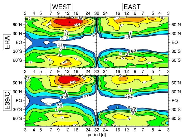
Forcing and propagation of planetary waves. To determine the properties of the generation of planetary waves, their propagation through the stratosphere and their role in the momentum budget of the stratosphere, i.e. the stratospheric response to planetary wave drag (PWD), an analysis of stationary planetary wave patterns (up to zonal wavenumber 8) at different altitudes between the free troposphere and the upper model layers is required. This diagnostic can be augmented by calculations of empirical orthogonal functions (EOFs) and of refractive index. Supplementary to the standard energy spectrum analysis, investigation of transient wave behaviour is necessary. Here, a wavenumber-frequency analysis (WFA) can help to resolve transient waves at distinct wavenumbers into standing and eastward and westward travelling waves at different frequencies (Hayashi, 1982). The WFA can be performed by using power-, co-, and quadrature spectra of the time spectral analysis methods such as the maximum entropy method, the direct Fourier transform method or the lag correlation method. An example is displayed in Figure 1. In order to determine the amplitudes and phases of the zonal quasi stationary planetary waves in the lower stratosphere, total ozone fields can be analysed by means of spectral statistical methods. Here, the total ozone column is considered as a conservative tracer to illuminate the variablity of wave structures in the lower stratosphere. To derive the wave parameters from the ozone distribution the spectral statistical technique Harmonic Analysis can be applied to each latitude which corresponds to an approximate deconvolution of the power spectrum. The spectral properties can further be used to gain two hemispheric Ozone Variability Indices which are defined as the hemispheric mean of the zonal amplitude of the planetary waves number 1 and 2. Stratospheric
response
to wave drag. Correlations of Eliassen-Palm fluxes (i.e.,
vertical
and meridional heat and momentum fluxes) with dynamical and chemical
fields
(e.g., temperature, wind speed, ozone) and parameters (e.g., size and
persistence
of the polar vortex, PSC potential) are necessary to investigate the
stratospheric
response to wave drag and its consequences for chemical and physical
processes
in CCMs (Newman et al., 2001; Austin et al., 2003).
Moreover, a check of the ability of CCMs to reproduce
correctly the
seasonality of the Brewer-Dobson circulation is needed. This can be
done
by calculations of cross sections of the residual circulation mass
streamfunction
(latitude vs. height), which are based on re-analyses (e.g., NCEP,
ERA-40)
and corresponding results derived from CCMs.
|
|
|
|
|
Derived diagnostic properties such as the relative roles of PWD and gravity wave drag (GWD) in polar downwelling, and seasonally dependent changes of low frequency behaviour of stratospheric chemistry (e.g., ozone loss in spring, absorbing aerosols) in coupled vs. uncoupled models must be checked. Quasi-Biennual
Oscillation
(QBO), Semi-Annual Oscillation (SAO). It is also important to
validate
the ability of CCMs to reproduce key oscillations in the stratosphere.
One such oscillation is the semi-annual oscillation (SAO) of equatorial
zonal winds at the stratopause. All CCMs simulate this to some extent,
but the realism of the models? SAOs varies considerably. CCMs are now
just
beginning to simulate the quasi-biennial oscillation (QBO), usually
through
the inclusion of enhanced GWD. It will be important to confirm that the
models are obtaining a QBO for the right reasons, and that the
extratropics
responds in the correct manner.
Transport in the stratosphere involves both meridional
overturning (the
residual circulation) and mixing, which together represent the
Brewer-Dobson
circulation. The most important aspects are the vertical mean motion
(diabatic
velocity) and the horizontal mixing. The horizontal mixing is highly
inhomogeneous,
with transport barriers in the subtropics and at the edge of the
wintertime
polar vortex; mixing is most intense in the wintertime ?surf zone? and
is extremely weak in the summertime extratropics. Accurate
representation
of this structure in CCMs is important for the ozone distribution
itself,
as well as for the distribution of chemical families that affect ozone
chemistry (NOy, Cly, H2O, CH4). Within both the tropics and the polar
vortex,
the key physical quantities to represent are the degree of isolation
and
the diabatic ascent or descent, respectively.
It is useful to distinguish between transport in the
stratospheric ?overworld?
and in the UTLS. In the stratospheric overworld, there is a reasonably
good understanding of the relevant processes and of how to quantify
them.
In contrast, the theoretical understanding of transport in the UTLS is
relatively poor. This presents a challenge to determining appropriate
diagnostics
for model-measurement comparison.
Subtropical
and
polar mixing barriers. With respect to the degree of isolation,
useful information can be obtained from instantaneous snapshots of
tracer
fields, which makes the model-measurement comparison straightforward.
For
this purpose there is a wealth of high-quality observational data
available.
A simple check on the degree of isolation is provided by the sharpness
of latitudinal gradients of long-lived species (CH4, N2O, CFC11).
However
since these gradients can be smeared out in zonal means, it is
important
to look at slices perpendicular to the mixing barrier (approximately,
but
not necessarily, at a single longitude). Equivalent latitude is an
effective
tool to create composites in the polar regions, but is probably not
viable
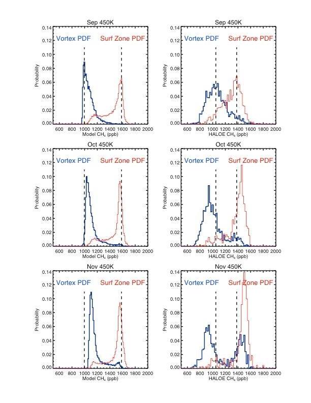
in the tropics. A way to avoid latitudinal smearing without relying on
equivalent latitude is to look at tracer probability distribution
functions
(PDFs) (see Figure 2), which allow a direct model-measurement
comparison.
The degree of isolation can be diagnosed in more detail from the
structure
of chemical correlations, though their interpretation is not always
straightforward.
Within the very lowest part of the overworld in the tropics, just above
the tropopause, where the tropical mixing barrier appears to be fairly
leaky, horizontal transport into midlatitudes can also be quantified by
the propagation of the annual cycle in CO2 and H2O, which has been well
observed in aircraft measurements. Finally, transport out of the
tropics
can also be quantified in terms of streamers, but the quantification
depends
on how the streamers are defined.
Diabatic ascent or descent has two aspects. First, a model
must have
the correct vertical residual velocity (or, equivalently, diabatic
heating
or cooling rates). This is controlled by the wave drag in the
stratosphere
and above. There are no direct measurements of these quantities, and,
hence,
they must be inferred from radiative calculations based on observed or
assimilated temperatures and radiatively active species. This
introduces
some uncertainties in the comparison. The second aspect is the impact
of
the vertical residual motion on the actual vertical motion of chemical
species. This depends on the degree of isolation. For example, if a
model
has spurious mixing across the vortex edge, then the descent of
chemical
species will reflect the diabatic descent in a broad region including
the
surf zone, rather than within the vortex. Assuming that the degree of
isolation
is correct, then it is possible to make a direct comparison between
models
and measurements by examining the ascent or descent rate of tracer
isopleths.
A well known example is the ascent rates of tropical H2O mixing ratios
which create the ?tape recorder? phenomenon in mixing ratio time series
plots.
Meridional
circulation.
The combined effect of the above processes determines the Brewer-Dobson
circulation. Both horizontal mixing and the residual circulation are
driven
in large measure by the momentum deposition (wave drag) from planetary
waves propagating from the troposphere into the stratosphere, with more
wave drag leading to a stronger Brewer-Dobson circulation in both
respects.
Because planetary waves can only propagate into the stratosphere when
the
winds are westerly, the Brewer-Dobson circulation is restricted to the
winter hemisphere. The wave drag is easily quantified from the net
planetary
wave flux into the stratosphere, nominally taken to be v?T? (vertical
EP
flux) at 100 hPa. The relationship between this wave flux and the
residual
circulation is quantified, through temperature, in the Dynamics
diagnostics
(see Table of Processes). With regard to chemical transport, the
seasonal
cycle of O3 in the extratropics exhibits a marked build-up during the
winter-spring
period due to the Brewer-Dobson circulation. Years with greater
planetary
wave flux also have a greater ozone build-up, a relationship that is
well
established from observations and provides a good diagnostic for CCM
validation.
The Brewer-Dobson circulation also determines the mean age of
air. Unfortunately,
the possibilities for direct comparison with data are more limited than
for the processes described above, because the measurement precision
requirements
are so stringent that, at present, only in-situ data can be used. This
particularly limits comparisons in the upper stratosphere.
Nevertheless,
in NASA?s Models and Measurements Intercomparison II, mean age of air
was
found to be a very powerful diagnostic for identifying model
deficiencies.
Mean age can be validated from measurements of long-lived species that
have linearly increasing concentrations (e.g., SF6, CO2). Propagation
of
the annual cycle of mean age can be validated from CO2 measurements in
the overworld (and H2O in the tropics). However other components of the
age spectrum (e.g., semi-annual, biennial) are very difficult to
validate.
UTLS
transport.
In contrast to the stratospheric ?overworld? discussed above, transport
in the UTLS region is far more complex. Yet many of the same concepts
appear
to be useful for validation. The extratropical tropopause is a barrier
to quasi-horizontal mixing, causing a significant contrast in many
chemical
species between the lowermost stratosphere and the troposphere. The
degree
of isolation can be assessed by the sharpness of vertical gradients at
the tropopause (vertical gradients because tropopause height changes
with
latitude), and with chemical correlations (e.g., O3 vs. CO). For the
former
there is plentiful ozonesonde data, and for the latter there is a
wealth
of aircraft data. These data are not sufficient to establish
climatologies,
but are nevertheless useful for process-based validation. However, it
is
important to compare models and measurements at similar longitudes,
because
there is significant longitudinal variation of the dynamical features
in
the UTLS (especially the tropopause). Unlike in the stratospheric
overworld,
UTLS transport is not quasi-zonal, and many chemical species are not
sufficiently
long-lived to be well-mixed longitudinally.
|
|
|
|
|
Radiation The representation of the radiation field is a crucial aspect
in CCMs
if ozone abundances and temperature changes are to be accurately
calculated
in the present and future atmosphere. Radiation affects CCMs through
photolysis
rate and heating rate calculations. Chemically active constituents,
such
as ozone, are strongly affected by photolysis rates, which are derived
from the radiation field. At the same time these trace gases feed back
on temperature and thus circulation through the radiative heating
rates.
At present most models calculate radiative heating rates and photolysis
rates in an inconsistent manner. For example, the spherical geometry of
the Earth might be included in the photolysis rate calculation, but not
in the heating rate calculation. Also different radiation schemes are
usually
employed for the two calculations. Ideally, such inconsistencies would
be avoided. However, here we evaluate these two calculations
separately.
|
|
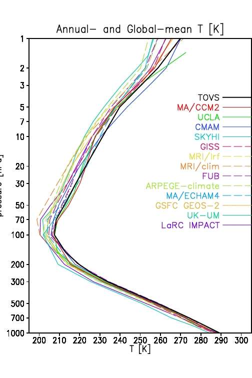
Figure 3: Long-term global-mean temperature climatology. Vertical structure of the long-term, annual global-mean temperature (K) from observations (thick black line) and 13 models (thin coloured lines). Observations are a 17-yr-mean (Pawson et al., 2000). |
|
|
Solar UV-visible photolysis in the stratosphere. Photolysis rates in the stratosphere control the abundance of many chemical constituents that in turn control the production and loss of ozone. A photolysis rate generally requires knowledge of the actinic fluxes at solar and UV-visible wavelengths (190-800 nm) as a function of altitude and solar zenith angle. Accurate calculations of these fluxes require accurate representation of scattering, albedo, and refraction. Particular concerns in photolysis rate calculations for the lower stratosphere are the effect of tropospheric cloudiness, which can significantly increase the rates for certain gases, and photolysis at solar zenith angles greater than 90°. Diagnostic parameters for photolysis rates in CCM model comparisons include the radiative transfer of UV-visible wavelengths and calculated rates for individual gases. Key variables in such model comparisons are the distributions of pressure, ozone, stratospheric aerosols, and tropospheric clouds. As a minimum test, the photolysis rates of O3 and NO2 should be stored as three-dimensional fields at local noon and compared to observations. In addition, actinic fluxes at the ground in different wavelength intervals should be compared. Radiative
heating
rates. The radiative heating rate calculation is the
fundamental
link between ozone and climate. As this calculation plays the central
part
in CCM feedbacks it is extremely difficult to separate cause and effect
in a fully coupled model. Radiative heating rate calculations can only
be truly evaluated in an offline comparison of radiation schemes.
Currently,
the lack of this comparison is one of the most important limitations in
understanding CCM differences and we strongly advocate such a
comparison
be initiated. A set of standardised background atmospheres and
radiation
scheme inputs should be compiled, along with a reference set of
calculations
from several state of the art line-by-line and scattering (e.g.,
Discrete-Ordinate)
models. These should then be made available to the community to
evaluate
their own CCM radiation scheme. Differences in radiative heating rates
and trace gas fields can then be used to evaluate differences between
the
globally averaged climatological temperature of CCMs and their
temperature
response to changes in greenhouse gases loadings and other
perturbations.
Radiative
heating
within an online framework. To evaluate radiative heating
within
an online framework the long-term global-mean temperature climatology
of
CCMs can be compared to observations (see Figure 3). An online
framework
allows a combined test of the model?s background atmosphere and
radiative
heating profile. Also, the globally averaged transient temperature
changes
over both a single year and the past ~25 years can be compared to
Stratospheric
Sounding Unit and Microwave Sounding Unit satellite observations. This
tests both the evolution of forcing agents, as well as the radiative
heating
and the radiative relaxation time in the model.
Stratospheric
Chemistry and Microphysics
Chemistry is clearly a natural process controlling the distribution of ozone in the atmosphere. Virtually all reaction rates are to a varying extent temperature dependent, providing one of the ways in which chemistry and dynamics are coupled. The importance of chemistry relative to other processes such as transport varies substantially depending on the local solar conditions as well as altitude. In the upper stratosphere transport plays a role by controlling the concentrations of the long-lived tracers such as active chlorine, but photochemical timescales are so short that transport has a minimal direct impact on ozone. However, in the lower stratosphere, the photochemical timescales are rather longer (typically of order months) and interactions with dynamics are complex and difficult to model accurately. Aerosols also may have an important role to play in the lower stratosphere since, in addition to their radiative impact, chemical reactions can take place within or on the particles and these reactions may lead to additional ozone depletion. Solar conditions are also important: for example, in polar night the distribution of chemical species is quite different to that in mid-latitudes where a clear diurnal variation in solar insolation occurs. Also, photochemical conditions are different in polar summer when the impact of the continuous daylight may be to photolyse the reservoir species entirely, depending on altitude. The different timescale of the processes in different parts of the atmosphere implies that a variety of modelling techniques can be effective. Photochemical
mechanisms
and short timescale chemical processes. In the list of processes for
stratospheric
chemistry and microphysics, one of the most important tasks is to
verify
the performance of the underlying photochemical mechanisms, including
the
computation of photolysis rates. Model comparisons of this sort need to
be completed using box model versions of the code used in the CCM,
looking
at timescales up to one week or so. Future studies can follow the
example
of the 'model and measurement tests' of Park et al. (1999). Very few
measurements
exist for direct comparison of photolysis rates (e.g., Gao et al.,
2001),
but there have been some attempts at inferring photolysis rates from
chemical
measurements. The comparisons could be made using the different model
calculations
for ozone loss and production in each of the catalytic cycles supported
by Lagrangian studies using observations from a wide range of sources
both
in situ and remote. Model diurnal variations could also be compared and
verified with a limited range of observations.
|
|
|
|
|
Long timescale chemical processes. The investigation of long timescale photochemical processes needs to be completed within the CCM itself as tracer transport has a significant impact. All the model chemical constituents need to be output three-dimensionally as well as the appropriate dynamical variables such as temperatures. One instantaneous ?snapshot? per month should be sufficient for the purpose of comparing the abundances of model reservoirs and precursors to the radicals which directly affect ozone. The inter-relations between long-lived tracers also need to be compared in detail with similar results determined from space-based or in-situ observations. Summer
processes and
polar processes in winter/spring. In the summer, the polar
regions
are a special case of atmospheric chemistry because of the continuous
or
near continuous daylight. These conditions have revealed some possible
discrepancies in NOx chemistry. This has an impact on ozone amounts
directly
in the polar regions and also in mid-latitudes via transport from the
polar
regions. In the winter/spring period, low temperatures lead to the
formation
of condensed matter and heterogeneous chemistry becomes important. Some
aspects of heterogeneous chemistry can be investigated in box model
simulations,
but because of the possible importance of denitrification and
dehydration,
as well as transport, a full three-dimensional model is required for a
complete analysis. Polar processes require an extensive set of chemical
and particle concentration values within the polar regions with daily
frequency.
One particular diagnostic, designed to address overall model ozone
depletion
in polar regions, requires the addition of a passive tracer to the CCM.
The tracer should be initialised on a specific date in the beginning of
the winter identically to the ozone on that day. Thereafter, assuming
that
model transport errors are negligible, the difference between the
photochemically
computed ozone and the passive tracer provides an indication of the
chemical
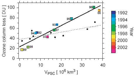
ozone loss. Observations (Rex et al., 2003) indicate that chemical
ozone
loss and Polar Stratospheric Cloud (PSC) volume are linearly correlated
(see Figure 4). Comparisons with this correlation would be a useful
test
of the ability of a model to simulate accurately the polar chemical
ozone
loss in the presence of PSCs.
Denitrification
&
Dehydration. Large polar ozone losses in both hemispheres occur
in winters that are sufficiently cold for denitrification and
dehydration
to occur. However the current representations of these processes in
CCMs
are simplistic, leading to large uncertainties in polar ozone loss and
in the impact on mid-latitudes. This is further complicated by (a) the
poor understanding of the mechanism by which denitrification occurs and
(b) CCM temperature biases in the polar vortex. The CCM representation
of denitrification can be investigated by analysing the key nitrogen
containing
species, NOy and HNO3, as a function of the well-conserved tracers N2O
and CH4. Remote and in situ data can be used to clarify these
relationships
and indicate any local loss in NOy or HNO3. Similarly the sum H2O + 2 x
CH4 is approximately conserved in the stratosphere, so significant
departures
would indicate dehydration or possibly settling from above.
Aerosol
processes.
Reactions involving sulphate aerosol are known to affect the production
and loss balance of stratospheric ozone. Not all CCMs are in a position
to investigate these processes in detail, as in some instances a
complete
sulphur reaction set is needed. Nonetheless, even for those models with
a passive sulphate amount, it would be of interest to complete
simulations
describing the impact of a major volcanic eruption such as that of Mt.
Pinatubo.
Aerosols
& Cloud
Microphysics. Aerosol and cloud related processes affect
the
whole UTLS region. There is a need to investigate these processes in
CCMs
and validate them using the available satellite and aircraft data. The
required model variables are liquid water and ice, temperature, and
aerosols,
and will be required at a relatively high spatial and temporal
frequency,
i.e., at least every three days and for every model grid point in the
UTLS
region. Further output of chemical constituents and potential vorticity
would be useful to examine heterogeneous chemistry and the dynamical
structure
of the tropopause.
The Way Ahead
Of the comprehensive suite of diagnostics for stratospheric CCMs listed in Table 1, several have been applied before to a range of models (Austin et al., 2003; Pawson et al., 2000; Park et al., 1999), but many have not. Some models need further development before the diagnostics can applied. Thus, while clearly desirable, it is a major task to perform all these diagnoses given the complexity of the CCMs and the often subtle changes under consideration. A step-wise approach is required to the use of the Table. In practice modeling groups need to develop their own priorities among these diagnostics. The choices will depend on the known strengths and weaknesses of each model, the processes and constituents already included, and the existing output from runs already performed. It will also depend on the scientific focus of each modeling group and the issue being addressed. For example, predictions of polar ozone loss will have more credibility if a model has been shown to compare well with diagnostics such as ozone loss versus VPSC, v?T?, and ClOx, NOy, etc. In this case, good performance against TTL diagnostics is less relevant. Over time each model will gradually increase the number of tests applied and overall confidence will increase. The lasting impact and the full benefit from the workshop will come from concerted validation activities based on the Table of Processes. In order for these activities to succeed over the next several years, broad support is needed from the atmospheric sciences community and its managers. It is important that the validation procedures and goals defined for these activities are accepted at the start and valued by all participants in this joint exercise. SPARC working groups are being set up so that real progress can be made in the next couple of years in time for the next WMO/UNEP and IPCC assessments. The SPARC GRIPS group is continuing the work on the comparisons for the dynamics issues. SPARC groups have been formed on CCM chemistry and radiation comparisons and they are defining plans for their issues. Updated information is available at http://www.pa.op.dlr.de/workshops/ccm2003/ together with the names of people coordinating the various activities. All scientists interested in participating should contact the appropriate coordinating scientist. To facilitate this process-oriented validation of CCMs, we intend to provide participants with access to diagnostic software packages. These routines will be archived in a central location. The goal in supplying such software is to simplify such activities as quality control of model output, calculation of more complex model diagnostics, statistical evaluation of model/data differences, and graphical display of results. Use of this software is not mandatory. Rather, the intent is to make it easier for groups to compute a broad range of calculations in a reasonably consistent way. Centralized software repositories have been of great benefit in other Model Intercomparison Programs (?MIPs?), such as the Atmospheric Model Intercomparison Project AMIP and the Coupled Model Intercomparison Project CMIP. These have freely supplied software for quality control of model output, data visualization, and interpolation of boundary condition datasets to a specific model grid. The CCM community can benefit from the experiences gained during previous model intercomparison exercises, particularly in terms of experimental design, definition of standard model output, and statistical aspects of model-data comparisons. Software developed in the course of previous MIPs, such as ?performance portraits? and Taylor diagrams, provide useful means of summarizing many different aspects of climate model performance. In collaboration with groups such as the Program for Climate Model Diagnosis and Intercomparison (PCMDI), we intend to modify these diagnostic tools in order to suit the specific needs of the CCM community. This suite of processes and diagnostics should become a
benchmark for
validation. Confidence in the performance of CCMs will increase as more
model attributes become validated against the whole suite of
diagnostics.
Further, new models can be evaluated against an acknowledged, benchmark
set of diagnostics as the models are developed. At the same time, the
diagnostics
themselves should develop as experience is gained and as new
measurements
become available allowing more processes to be diagnosed. It is hoped
that
this workshop has laid the groundwork to a more comprehensive approach
to CCM validation which will be developed by all scientists who become
involved, irrespective of whether they attended the workshop or not.
Acknowledgements We wish to thank all the agencies that supported this
workshop. The
workshop was held under the auspices of the Institute for Atmospheric
Physics
of the German Aerospace Center (DLR), the EU research cluster OCLI
(Ozone
CLimate Interactions), and SPARC.
References
Austin, J., D. Shindell, S.R. Beagley, C. Brühl, M. Dameris, E. Manzini, T. Nagashima, P. Newman, S. Pawson, G. Pitari, E. Rozanov, C. Schnadt, and T.G. Shepherd, Uncertainties and assessments of chemistry-climate models of the stratosphere, Atmos. Chem. Phys., 3, 1-27, 2003. Eyring V., N.R.P. Harris, M. Rex, T.G. Shepherd, D.W. Fahey, J. Austin, M. Dameris, H. Graf, T. Nagashima, and B. Santer, Brief report on the Workshop on Process-Oriented Validation of Coupled Chemistry-Climate Models, SPARC Newsletter no. 22, 2004 Gao, R.S., E.C. Richard, P.J. Popp, G.C. Toon, D.F. Hurst, P.A. Newman, J.C. Holecek, M.J. Northway, D.W. Fahey, M.Y. Danilin, Observational evidence for the role of denitrification in Arctic stratospheric ozone loss, Geophys. Res. Let., 28, 15, 2879-2882, 2001 Gibson, J.K., P. Kallberg, S. Uppala, A. Hernandez, A. Nomura, and E. Serrano, ERA description, ECMWF Re-Analysis Project Report Series, 1, 1-72, 1997. Hayashi, Y., Space-time spectral analysis and its applications to atmospheric waves, J. Meteor. Soc. Japan, 60, 156-171, 1982. Hein, R., M. Dameris, C. Schnadt, C. Land, V. Grewe, I. Koehler, M. Ponater, R. Sausen, B. Steil, J. Landgraf, C. Bruehl, Results of an interactively coupled atmospheric chemistry-general circulation model: Comparison with observations, Ann. Geophysicae, 19, 435-457, 2001. Newman, P.A., E.R. Nash, J.E. Rosenfield, What controls the temperature of the Arctic stratosphere during spring?, J. Geophys. Res., 106, 19999-20010, 2001. Park J.H., M.K.W. Ko, C.H. Jackman, R.A. Plumb, J.A. Kaye, K.H. Sage, Models and Measurements Intercomparison II, NASA/TM-1999-209554, 1999. Pawson, S., K. Kodera, K. Hamilton, T.G. Shepherd, S.R. Beagley, B.A. Boville, J.D. Farrara, T.D.A. Fairlie, A. Kitoh, W.A. Lahoz, U. Langematz, E. Manzini, D.H. Rind, A.A. Scaife, K. Shibata, P. Simon, R. Swinbank, L. Takacs, R.J. Wilson, J.A. Al-Saadi, M. Amodei, M. Chiba, L. Coy, J. de Grandpre, R.S. Eckman, M. Fiorino, W.L. Grose, H. Koide, J.N. Koshyk, D. Li, J. Lerner, J.D. Mahlman, N.A. McFarlane, C.R. Mechoso, A. Molod, A. O'Neill, R.B. Pierce, W.J. Randel, R.B. Rood, F. Wu: The GCM-Reality Intercomparison Project for SPARC: Scientific Issues and Initial Results, Bull. Am. Meteorol. Soc., 81, 781-796, 2000. Rex, M., R.J. Salawitch, P. von der Gathen, N.R.P. Harris, M. Chipperfield, B. Naujokat, Arctic ozone loss and climate change, Geophysical Research Letters, in press, 2004. WMO, Scientific Assessment of Ozone Depletion: 2002, Global
Ozone
Research and Monitoring Project - Report No. 47, 498 pp, Geneva, 2003.
|
go to:
top of the table top of the text