| Prof. Dr. habil. Veronika Eyring
Head of
Earth System Model Evaluation and Analysis Departement |
and: Professor and Chair of Climate Modelling University of Bremen Institute of Environmental Physics (IUP) Otto-Hahn-Allee 1 28359 Bremen, Germany Phone: +49-421-218-62733 http://www.iup.uni-bremen.de/
Scopus Author ID: 13402933200 |

|
 |
Advanced Earth System Model Evaluation for CMIP (EVal4CMIP) - Accounting for observational uncertainties and internal climate variability using satellite data – Project funded under the top female researchers W3 programme through the Initiative and Networking Fund of the Helmholtz Society
|
 |
|
Project Coordinator and Contact DLR: Prof. Dr. habil. Veronika Eyring Deutsches Zentrum für Luft- und Raumfahrt (DLR) Institute of Atmospheric Physics Oberpfaffenhofen 82234 Wessling, Germany Email: Veronika.Eyring@dlr.de www: http://www.pa.op.dlr.de/~VeronikaEyring/
|
In Cooperation with
University of Bremen Institute of Environmental Physics
Otto-Hahn-Allee 1
|

01.09.2017 - 31.08.2022
2 EXPOSE
The evaluation of Earth system models (ESMs) with observations is crucial for model improvements and a better process understanding of the climate system. It is also a vital prerequisite for trustworthy climate projections of the 21st century to be used for policy guidance. High-profile reports such as the Intergovernmental Panel on Climate Change Fifth Assessment Report (IPCC AR5) attest to the exceptional societal interest in understanding and projecting future climate. The climate projections considered in the most recent report are mostly from the ESM experiments defined and internationally coordinated as part of the Coupled Model Intercomparison Project Phase 5 (CMIP5). CMIP has been a major, very successful endeavour of the climate community for understanding past climate changes and for making projections and uncertainty estimates of the future in a multi-model framework. However, adequate use of CMIP results requires an awareness of the limitations. It is essential, therefore, to subject models to a systematic evaluation against observations.
While progress has been made in ESM evaluation over the last decades, there are important opportunities and challenges for CMIP6, with simulations starting in 2016. A critical aspect in ESM evaluation is the availability of consistent, error-characterized global and regional Earth observations as well as accurate global reanalyses that are constrained by assimilated observations. In many cases the lack or insufficient quality of long-term observations or observations for process evaluation remains an impediment, but improvements can be made by fully exploiting existing observations and by better taking into account observational uncertainty. Part of the difference between model results and observations can be attributed to unforced variability, originating from the nonlinear nature of the variable climate system. An accurate assessment of model performance therefore has to take into account internal climate variability in addition to observational uncertainty. Another longstanding open scientific question is the missing relation between model performance and future projections. While evaluation of the evolving climate state and processes can be used to build confidence in model fidelity, this does not guarantee the correct response to changed forcing in the future. The relatively new field of emergent constraint analysis which refers to the use of observations to constrain a simulated future Earth system feedback offers the potential to reduce uncertainty in climate projections.
The goal of EVal4CMIP is to address the main outstanding scientific issues in ESM evaluation listed above by (a) exploiting available satellite observations and developing new evaluation methods that take into account observational uncertainty, (b) better consideration of internal climate variability in ESM evaluation, and (c) identifying critical processes most important to the magnitude and uncertainty of future projections. Our starting point for observations used in the evaluation of CMIP models will be datasets that are made available as part of obs4MIPs (Observations for Model Intercomparison Projects) that are technically aligned with CMIP model output as well as long-term data products for example from the ESA Climate Change Initiative (CCI). While one focus of our work is the broad characterization of the CMIP models across the atmosphere, ocean, and terrestrial domains, observational uncertainty, internal variability and emergent constraints will be studied for specific applications focusing on carbon dioxide (CO2), methane (CH4), and sea ice. Here, we will use mainly products that are developed at the DLR Institute of Atmospheric Physics (DLR-IPA) and the Institute of Environmental Physics and Remote Sensing of the University of Bremen (IUP-IFE) to further explore the impact of observational uncertainty and internal variability on evaluation results and emergent constraints, and to develop corresponding statistical methods. Example datasets include the ESA CCI CO2 and CH4 products and sea ice datasets from passive microwave sensors such as the Advanced Microwave Scanning Radiometer - Earth Observing System (AMSR-E). New datasets such as those from the French / German Climate Methane Remote Sensing Lidar Mission (MERLIN) and ESA’s Sentinel 5 Precursor mission will be included as soon as the data become available. The starting point for CO2 for example will be the analysis of surface fluxes and concentration anomalies particularly with respect to feedbacks with other geophysical quantities such as surface temperature. We will also invest in operational evaluation of physical and biogeochemical aspects by contributing the new methods and diagnostics developed in EVal4CMIP to the Earth System Model Evaluation Tool (ESMValTool). The ESMValTool is a community-wide diagnostic tool for the evaluation of ESMs against observations that is developed by various international partners under the lead of the applicant at DLR-IPA. The advanced version of the ESMValTool will be applied to CMIP models and the ECHAM/MESSy Atmospheric Chemistry (EMAC) model, which is now the main modelling tool at DLR-IPA.
Our work is expected to make a substantial contribution to CMIP6 which will support the next IPCC Assessment Report with simulations and new results on the state of scientific knowledge relevant to climate change. The studies on emergent constraints will be used to draw conclusions for critical questions such as allowable CO2 emissions for a specific temperature target. Our studies will help reducing overall uncertainty of future climate estimates while targeting model development onto phenomena underpinning the magnitude and uncertainty of future Earth system change.
The suggested research plan builds on the successful collaboration and expertise gained within the Helmholtz-University Young Investigators Group SeaKLIM ‘Impact of Ship Emissions on Atmosphere and Climate’ led by the applicant. The SeaKLIM team has established a strong research link and an active cooperation between DLR-IPA and IUP-IFE. Within EVal4CMIP we will continue to exploit synergies in the areas of Earth system modelling and Earth observations at DLR-IPA and IUP-IFE through close cooperation between experts in both areas, to tackle some of the key challenges in ESM evaluation. A cooperative W3 professorship will foster continuous research success, will strengthen future cooperation, and will be a major step forward in the applicant’s career.
3 Eval4CMIP Results and Milestone Descriptions
M0.1 Webpage
The webpage for Eval4CMIP is available at: http://www.pa.op.dlr.de/%7EVeronikaEyring/EVal4CMIP.html
M1.2 Initial assessment of CMIP6 models and EMAC with a focus on CO2, CH4, and sea ice
The evaluation of EMAC was not possible because runs are not available, we thus focused on other CMIP6 models instead.
Carbon Dioxide
There were large uncertainties in simulating atmospheric CO2 concentrations in earth system models (ESMs) participating in CMIP5. Several models saw a focus on improving on the carbon cycle and its components going into CMIP6. Gier et al. (2020) focuses on column-averaged CO2 to compare emission driven simulations of both CMIP5 and CMIP6 models with a spatially resolved satellite dataset over the time range 2003-2014.
CMIP6 models on average overestimate the CO2 content in the atmosphere (see the offsets in Figure 1), owing to a slight overestimation of the yearly CO2 growth rate. However, they capture the seasonal cycle and its increase with increasing latitude quite well. Due to the comparison with satellite data, which naturally features missing data due to external factors like cloud coverage, the simulations were sampled like the data. This resulted in solving a previously thought discrepancy where the seasonal cycle amplitude in the northern midlatitudes shows a strong negative trend in the satellite data, while the multi-model mean shows a non-significant positive trend. Gier et al. (2020) were able to attribute this to the different spatial sampling of the two satellites, which overlapped but neither covered the full time range, contributing to the observational dataset, which introduced an artificial negative trend. Overall, the CMIP6 ensemble shows a slightly better agreement with the satellite data than the CMIP5 ensemble, signifying an overall improvement in the models.
Figure 1: Comparison of time series from satellite column-averaged CO2 (XCO2) (black), CMIP6 multi-model mean XCO2 (orange) and surface CO2 (red), and NOAA surface CO2 station data (blue) at selected sites, with the coordinates noted in brackets above the time series and the altitudes shown in the map plot. The multi-model mean for both XCO2 and surface CO2 was offset to have the same average value as the satellite XCO2 for better comparison, and this offset is noted above each time series. From Gier et al. (2020).
Sea ice
The decline in Arctic sea ice thickness and extent contributes to the rise of global temperatures through the ice-albedo feedback. An evaluation of the sea ice extent (SIE) is therefore an important factor when assessing the robustness of climate projections from models. Here, the results from Lauer et al. (2017) and Senftleben et al. (2020) based on CMIP5 data are shown, an evaluation of sea ice in CMIP6 is not available, yet. In this analysis, SIE has been calculated by adding up the surface area of all grid cells with a sea ice concentration equal or larger than 15%. As an example, the time series of September Arctic sea ice extent in Figure 3 shows that the spread between the four observational data sets (thick black lines) from ESA CCI and NSIDC is much smaller than the spread among the CMIP5 models (coloured lines), which amounts to about 9 million km2 between CSIRO-Mk3-6-0 (largest positive bias) and GISS-E2-H (largest negative bias). Most of the time, the CMIP5 multi-model mean (thick red line) lies within the observational spread although the RCP4.5 simulation that has been used to extend the historical simulations beyond 2005 does not show the decrease in sea ice extent that has been observed between 2005 and 2013. The negative trend over the observed time period from 1990 to 2010 is about 1 million km2 per decade in all four observational data sets. The magnitude of this trend is, however, underestimated by the CMIP5 multi-model mean (Lauer et al. 2017).
Figure 3: Evolution (1960–2020) of September Arctic sea ice extent in million km2 from the CMIP5 models (coloured lines) and from observations (thick black lines). The pole holes of the satellite data sets have been filled assuming a sea ice concentration of 100%. All available ensemble members from a given model are shown and drawn in the same colour as indicated in the legend. The CMIP5 multi-model mean is shown in bold red and the grey shading shows the standard deviation of the CMIP5 ensemble. From Lauer et al. (2017).
As a second example, Figure 4 shows trend distributions for Arctic SIE that were calculated over the whole 34-year time period from the results of 29 CMIP5 models and from a large initial condition ensemble obtained with the Community Earth System Model (CESM LE). Here, the assumption is that the spread in large initial condition ensembles (round-off level perturbation) represents the internal variability of the climate system within the context of a particular climate model. Comparing the standard deviation of the CMIP5 trends to the one obtained from the CESM LE gives an estimate of the impact of internal variability on the spread in the CMIP5 SIE trends. For SIE, the standard deviation of the CESM LE trends (0.21) is slightly smaller than one of the CMIP5 trends (0.27), suggesting that internal variability is an important but not the only factor determining the spread in the CMIP5 SIE (Senftleben et al. 2020).
Figure 4: Frequency distributions of the trend in sea ice extent calculated (left) from 29 CMIP5 models and (right) from the 38-member CESM LE over the time period 1979–2012. The red vertical lines represent the trend from NSIDC-NT observations. The values for the mean and the variance (sigma) of each trend distribution are given at the top of each panel. From Senftleben et al. (2020).
M2.2 Report on improved consideration of observational uncertainty in ESM evaluation for CO2, CH4, and sea ice
Observational uncertainties are commonly considered in model evaluation by comparing against multiple observational datasets as done e.g. in Bock et al. (2020). In this paper, the models are compared against a reference dataset and if available also against an alternative reference dataset. In order to go beyond this rather simple approach, so-called multi-observational climatologies have been introduced in the ESMValTool that can be used as reference datasets. Here, observational uncertainty of annual climatologies is estimated on a per-pixel basis by calculating the standard deviation of all years (annual average) from individual observational datasets against the multi-observational mean climatology. This standard deviation is then averaged over all observational datasets using the same weight for each dataset independent of its record length. The average includes the year to year variability and is then used as an estimate for the combined observational uncertainty. If the absolute differences between a model and the multi-observational climatology exceed this uncertainty estimate, the corresponding areas are stippled. Additionally, in the case of CO2, the observational uncertainty of the satellite dataset used in Gier et al. (2020) is less than 1 ppmv, accounting for both statistical uncertainties of individual soundings and uncertainties arising from regional and temporal biases. This is small enough that it can be neglected beside the much larger inter-model differences in CMIP6.
M3.2 Report on improved consideration of internal climate variability in ESM evaluation for CO2, CH4, and sea ice
To consider internal variability, the Climate Variability Diagnostics Package (CVDP, http://www.cesm.ucar.edu/working_groups/CVC/cvdp/) developed by NCAR’s Climate Analysis Section has been implemented into the ESMValTool (Eyring et al. 2020) through the recipe recipe_cvdp.yml. The CVDP allows the evaluation of the major modes of climate variability, including El Niño-Southern Oscillation (ENSO), Pacific Decadal Oscillation (PDO), Atlantic Multi-decadal Oscillation (AMO), and Atlantic Meridional Overturning Circulation (AMOC), as well as atmospheric teleconnection patterns like the Northern and Southern Annular Modes (NAM and SAM), North Atlantic Oscillation (NAO), and Pacific North and South American (PNA and PSA) patterns. While the temporal sequences of internal variability in models do not necessarily need to match those in the single realization of nature, their statistical properties (e.g. timescale, autocorrelation, spectral characteristics, and spatial patterns) need to be realistically simulated for credible climate projections. To evaluate this, CVDP provides plots of time series, spatial pattern, and power spectra of the modes of climate variability, and teleconnection pattern. Figure 6 shows the representation of ENSO teleconnections during the peak phase (December–February), showing that the different models produce a wide range of ENSO teleconnections.
Another possible way of considering internal variability is to use multiple ensemble members for each model and comparing the results. In Gier et al. (2020) this was done for CO2 by comparing the timeseries, growth rate and seasonal cycle amplitude for all available ensemble members for emission driven historical simulations (Figure 7). Models with multiple ensemble members available were ACCESS-ESM1-5 (3 members), CanESM5 (9 members), CanESM5-CanOE (3 members), MIROC-ES2L (3 members), MPI-ESM1-2LR (10 members). The timeseries for the different ensemble models cluster together and the ensembles differences are small compared to inter-model differences.
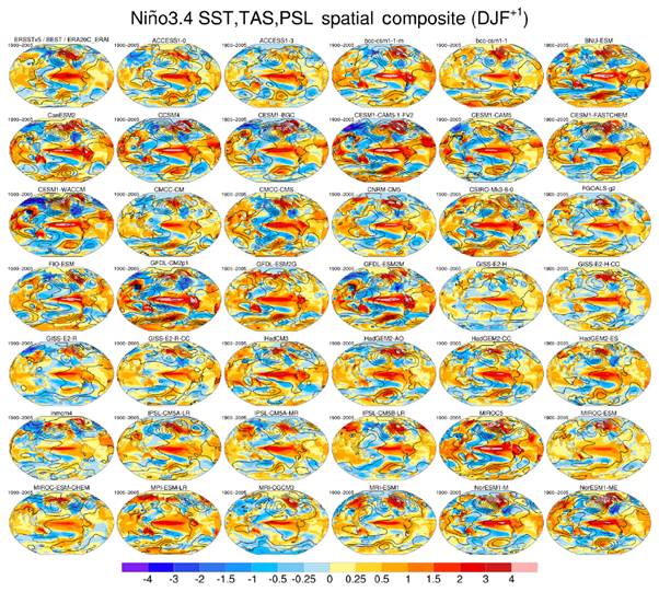
Figure 6: Global ENSO teleconnections during the peak phase as simulated by 41 CMIP5 models (see panel title) and observations (first row, upper left panel) for the historical period (1900–2005 for models and 1920–2017 for observations). These patterns are based on composite differences between all El Niño events and all La Niña events (using a standard deviation based threshold of the Niño 3.4 SST Index) occurring in the period of record. Colour shading denotes sea surface temperature and near-surface air temperature (°C), and contours denote sea level pressure with an interval of 2 hPa, with negative values dashed. The period of record is given in the upper left of each panel. Observational composites use ERSSTv5 for sea surface temperature, BEST for near-surface air temperature, and ERA20C updated with ERA-Interim for sea level pressure. Figure from Eyring et al. (2020), produced with recipe_cvdp.yml.
Figure 7: Global time series of monthly mean column-averaged carbon dioxide (XCO2) from 2003 to 2014 for emission-driven CMIP6 model simulations in comparison to satellite XCO2 data (bold black line). The model output is sampled as the satellite data. The top panels show the time series, while the middle panels show the computed monthly growth rate, which has been used to detrend the data to obtain the seasonal cycle shown in the bottom panel. All available ensemble members for each model are shown. From Gier et al. (2020).
M4.2 Report on observational constraints of future CO2 projections
Uncertainties in future climate projections of Earth system model (ESM) ensembles like the Coupled Model Intercomparison Project Phases 5 (CMIP5, Taylor et al. 2012) or 6 (CMIP6, Eyring et al. 2016) are high. Substantial contributions come from model uncertainties in carbon cycle feedbacks and associated atmosphere-land and atmosphere-ocean CO2 fluxes (Arora et al. 2020). Since these CO2 fluxes determine the fraction of anthropogenic CO2 emissions that stay in the atmosphere and act as greenhouse gas, precise projections of these fluxes are necessary to accurately assess policy-relevant climate metrics like the transient climate response to cumulative carbon emissions (TCRE) and remaining carbon budgets to reach specific warming targets.
The largest flux of the terrestrial carbon uptake is gross primary production (GPP) defined as the production of carbohydrates by photosynthesis. Elevated atmospheric CO2 concentration is expected to increase GPP in the future (“CO2 fertilization effect”). In a recent study, Schlund et al. (2020) present a two-step machine learning–based climate model weighting framework that combines an existing emergent constraint with a machine learning approach to constrain the spatial variations of multi-model projections of GPP.
In a first step (Step 1), Schlund et al. (2020) use an emergent constraint approach on CO2 fertilization from Wenzel et al. (2016) to constrain the global mean fractional change in GPP over the 21st century in the emission-driven Representative Concentration Pathway (RCP) 8.5 scenario. The technique of emergent constraints offers the possibility to reduce uncertainties in climate projections and can help guide model development by highlighting processes that are crucial to explaining the magnitude and spread of the modelled future climate change. Emergent constraints utilize an ensemble of ESMs together with observational data to constrain a simulated future Earth system feedback. In this first step, Schlund et al. (2020) find a global mean GPP increase (averaged over the period 2091-2100 relative to 1991-2000) of 39 ± 7%, which translates to a global mean GPP at the end of the 21st century of 171 ± 12 GtC yr−1 (the corresponding unconstrained CMIP5 inter-model range is compared to the unconstrained model range of 156-247 GtC yr−1).
In a second step, a machine learning model is used to constrain gridded future absolute GPP (Step 2a) and gridded fractional GPP change (Step 2b) in two independent approaches. For this, observational data products are fed into the machine learning algorithm that has been trained on CMIP5 data to learn relationships between present‐day physically relevant diagnostics and the target variable. The results for the end of the 21st century GPP distributions are illustrated in Figure 8, which shows an increased GPP change in northern high latitudes compared to regions closer to the equator. In a leave‐one‐model‐out cross‐validation approach, the machine learning model shows superior performance to the CMIP5 ensemble mean. Schlund et al. (2020) conclude that novel machine learning techniques are a promising avenue forward for such multivariate approaches and for constraining uncertainties in multi-model projections.
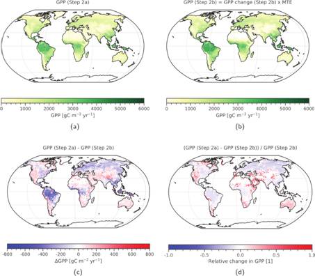
Figure 8 (top row): Absolute future GPP at the end of the 21st century (2091-2100) calculated using (a) Step 2a (absolute GPP) and (b) Step 2b (fractional GPP change). Both approaches give similar results, with global averages of (a) 169 GtC yr−1 and (b) 175 GtC yr−1, which are both consistent with the global result of Step 1 (171 ± 12 GtC yr−1). The pattern correlation between both approaches is R2 = 0.97. Bottom row: Absolute (c) and relative (d) differences between panels (a) and (b). From Schlund et al. (2020)
M4.3 Report on observational constraints of future CH4 projections
So far, CMIP6 models don’t include free-running CH4 emissions (Thornhill et al. 2021), therefore we cannot apply similar methods to constrain the future CH4 as for GPP. Other future constraints included into the ESMValTool include the constrain of future Indian Summer Monsoon projections based on present day precipitation (Lauer et al. 2020).
M4.4 Report on observational constraints of future sea ice projections
Weighting of multi-model projections has the potential to narrow uncertainties in climate model projections by moving beyond ‘model democracy’, i.e. not treating all models as equally likely to be true. As one method, multiple diagnostic ensemble regression (MDER) can be used to produce model weights by calculating the regression of historical diagnostics and a future parameter from ESM simulations. The model weights are then used to obtain a weighted multi-model mean with a reduced model uncertainty compared with the unweighted multi-model mean. MDER-calculated model weights can reduce the model uncertainty in CMIP5 projections of the Arctic sea ice extent by 30 to 50% (Figure 9). Compared to the unweighted multi-model mean, MDER results in an earlier year of near-disappearance of Arctic sea ice by more than a decade for the RCP8.5 scenario (Senftleben et al. 2020).
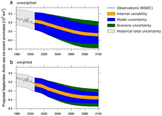
Figure 9: Total uncertainty in sea ice projections separated into the components internal variability (orange), model uncertainty (blue) and scenario uncertainty (green) estimated from 29 CMIP5 models (RCP4.5 and RCP8.5). Panels a and b show time series (1979-2100) of the uncertainties from unweighted and from MDER-weighted projections of sea ice anomalies, respectively. The gray shading shows the total uncertainty of the historical simulations, observations from the National Snow and Ice Data Center are shown as black lines. From Senftleben et al. (2020).
Literature
Arora, V.K., Katavouta, A., Williams, R.G., Jones, C.D., Brovkin, V., Friedlingstein, P., Schwinger, J., Bopp, L., Boucher, O., Cadule, P., Chamberlain, M.A., Christian, J.R., Delire, C., Fisher, R.A., Hajima, T., Ilyina, T., Joetzjer, E., Kawamiya, M., Koven, C.D., Krasting, J.P., Law, R.M., Lawrence, D.M., Lenton, A., Lindsay, K., Pongratz, J., Raddatz, T., Seferian, R., Tachiiri, K., Tjiputra, J.F., Wiltshire, A., Wu, T.W., & Ziehn, T. (2020). Carbon-concentration and carbon-climate feedbacks in CMIP6 models and their comparison to CMIP5 models. Biogeosciences, 17, 4173-4222
Bock, L., Lauer, A., Schlund, M., Barreiro, M., Bellouin, N., Jones, C., Meehl, G.A., Predoi, V., Roberts, M.J., & Eyring, V. (2020). Quantifying Progress Across Different CMIP Phases With the ESMValTool. Journal of Geophysical Research-Atmospheres, 125
Eyring, V., Bock, L., Lauer, A., Righi, M., Schlund, M., Andela, B., Arnone, E., Bellprat, O., Brotz, B., Caron, L.P., Carvalhais, N., Cionni, I., Cortesi, N., Crezee, B., Davin, E.L., Davini, P., Debeire, K., de Mora, L., Deser, C., Docquier, D., Earnshaw, P., Ehbrecht, C., Gier, B.K., Gonzalez-Reviriego, N., Goodman, P., Hagemann, S., Hardiman, S., Hassler, B., Hunter, A., Kadow, C., Kindermann, S., Koirala, S., Koldunov, N., Lejeune, Q., Lembo, V., Lovato, T., Lucarini, V., Massonnet, F., Muller, B., Pandde, A., Perez-Zanon, N., Phillips, A., Predoi, V., Russell, J., Sellar, A., Serva, F., Stacke, T., Swaminathan, R., Torralba, V., Vegas-Regidor, J., von Hardenberg, J., Weigel, K., & Zimmermann, K. (2020). Earth System Model Evaluation Tool (ESMValTool) v2.0-an extended set of large-scale diagnostics for quasi-operational and comprehensive evaluation of Earth system models in CMIP. Geoscientific Model Development, 13, 3383-3438
Eyring, V., Bony, S., Meehl, G.A., Senior, C.A., Stevens, B., Stouffer, R.J., & Taylor, K.E. (2016). Overview of the Coupled Model Intercomparison Project Phase 6 (CMIP6) experimental design and organization. Geoscientific Model Development, 9, 1937-1958
Gier, B.K., Buchwitz, M., Reuter, M., Cox, P.M., Friedlingstein, P., & Eyring, V. (2020). Spatially resolved evaluation of Earth system models with satellite column-averaged CO2. Biogeosciences, 17, 6115-6144
Lauer, A., Eyring, V., Bellprat, O., Bock, L., Gier, B.K., Hunter, A., Lorenz, R., Perez-Zanon, N., Righi, M., Schlund, M., Senftleben, D., Weigel, K., & Zechlau, S. (2020). Earth System Model Evaluation Tool (ESMValTool) v2.0-diagnostics for emergent constraints and future projections from Earth system models in CMIP. Geoscientific Model Development, 13, 4205-4228
Lauer, A., Eyring, V., Righi, M., Buchwitz, M., Defourny, P., Evaldsson, M., Friedlingstein, P., de Jeu, R., de Leeuw, G., Loew, A., Merchant, C.J., Muller, B., Popp, T., Reuter, M., Sandven, S., Senftleben, D., Stengel, M., Van Roozendael, M., Wenzel, S., & Willen, U. (2017). Benchmarking CMIP5 models with a subset of ESA CCI Phase 2 data using the ESMValTool. Remote Sensing of Environment, 203, 9-39
Schlund, M., Eyring, V., Camps-Valls, G., Friedlingstein, P., Gentine, P., & Reichstein, M. (2020). Constraining Uncertainty in Projected Gross Primary Production With Machine Learning. Journal of Geophysical Research-Biogeosciences, 125
Senftleben, D., Lauer, A., & Karpechko, A. (2020). Constraining Uncertainties in CMIP5 Projections of September Arctic Sea Ice Extent with Observations. Journal of Climate, 33, 1487-1503
Taylor, K.E., Stouffer, R.J., & Meehl, G.A. (2012). An Overview of Cmip5 and the Experiment Design. Bulletin of the American Meteorological Society, 93, 485-498
Thornhill, G., Collins, W., Olivi, D., Skeie, R.B., Archibald, A., Bauer, S., Checa-Garcia, R., Fiedler, S., Folberth, G., Gjermundsen, A., Horowitz, L., Lamarque, J.F., Michou, M., Mulcahy, J., Nabat, P., Naik, V., O'Connor, F.M., Paulot, F., Schulz, M., Scott, C.E., Seferian, R., Smith, C., Takemura, T., Tilmes, S., Tsigaridis, K., & Weber, J. (2021). Climate-driven chemistry and aerosol feedbacks in CMIP6 Earth system models. Atmospheric Chemistry and Physics, 21, 1105-1126
Wenzel, S., Cox, P.M., Eyring, V., & Friedlingstein, P. (2016). Projected land photosynthesis constrained by changes in the seasonal cycle of atmospheric CO2. Nature, 538, 499-+
| Back to Veronika Eyring's Homepage |