Expressed by formulae, this reads:
P_RHi(u) = a exp(-au) in the lowermost stratosphere
P_Si(s) = b exp(-bs) in tropospheric ISSRs
where a, b are constants, RHi is relative humidity wrt ice, Si is supersaturation with respect to ice, and u, s are variables on the RH and Si axes, respectively. P means probability density.
Cloud cleared Microwave Limb Sounder (MLS) data of upper tropospheric humidity on the 215 hPa pressure level have been evaluated in the same way to determine the global statistics of relative humidity with respect to ice. In agreement with the MOZAIC study we find that in the lowermost stratosphere the probability to get a certain value of relative humidity decreases exponentially with the relative humidity. In the Antarctic data class (data south of 55°S, mainly winter data) we also find an exponential distribution for RHi but with less steep slope. There is no change in the slope of the exponential distribution function at ice saturation. In the upper troposphere there are corresponding exponential distributions for RHi in ISSRs and in subsaturated regions (for 20%<RHi<100%), however with different slopes, viz. a steeper one in ice-supersaturated regions. In the cases of the tropospheric and antarctic data there is no indication of homogeneous ice nucleation at high humidities of RHi >150%, and the exponential distributions extend without change of slope up to 180-200%. Such extreme humidity events occur mostly in the tropics and at the edge of Antarctica. Their origin is currently unknown (maybe incidental lack of aerosol).
The following figures show mean values and standard deviations of temperatures and specific humidities inside ISSRs (bullets) and outside - i.e. in subsaturated air (open circles).
This indicates two different sources or
formation mechanisms of ISSRs, namely:
(1) adiabatic cooling of an airmass leads
to supersaturation (this seems not to be important in the tropics,
since the temperatures are very close together);
(2) moisture advection leads to supersaturation.
The largest ISSRs we have found in the MOZAIC data have pathlengths exceeding 1000 km. One example is shown in the next figure.
The yellow line marks the flight path of
a MOZAIC flight from Frankfurt, Germany to a location near Rio de Janeiro,
Brasil. Look at the part close to the northwest African coast. The flight
path is there parallel to a warm front that is approaching Africa. This
is where we have found the huge ISSR (more than 3000 km flight in supersaturated
air). In front of the front air is slowly uplifting and adiabatically cooling.
A certain distance to the east from the front and from the flight trajectory
one can see the clouds that form in the cooling air. This flight was therefore
in a supersaturated airmass, that was however at the flight position not
yet sufficiently moist for cirrus formation. The cooling necessary for
cirrus formation was only reached further to the east.
Vertical extensions could be obtained from radiosonde data from the Meteorological Observatory in Lindenberg, Germany. Unfortunately, this data set does not allow to distinguish between data in clear air (proper ISSRs) and in cloudy air (improper ISSRs). In spite of this, the statistics show up two regimes, one of which can be attributed to cirrus clouds and the other probably to ISSRs. This can be seen when the data are plotted on a so-called Weibull plot.
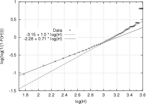 A Weibull plot is constructed in such a way, that random numbers drawn from
a Weibull distribution lie on a straight line. The slope of the line is
the power in the expression of the Weibull distribution. In our case the
data are located on two straight lines which cross at a height of 1000
m. The data points referring to larger vertical extensions are probably
taken inside cirrus clouds, which are typically thicker in the vertical
than 1000 m. The slope of the line in this part is 1.0, which means that
the Weibull distribution here is simply an exponential distribution. The
other part of the plot, i.e. H < 1000 m, probably contains data from
true ISSRs and perhaps sub-visible cirrus. The mean height in this regime
is about 500 m. This is also a characteristic vertical extension of sub-visible
cirrus clouds.
A Weibull plot is constructed in such a way, that random numbers drawn from
a Weibull distribution lie on a straight line. The slope of the line is
the power in the expression of the Weibull distribution. In our case the
data are located on two straight lines which cross at a height of 1000
m. The data points referring to larger vertical extensions are probably
taken inside cirrus clouds, which are typically thicker in the vertical
than 1000 m. The slope of the line in this part is 1.0, which means that
the Weibull distribution here is simply an exponential distribution. The
other part of the plot, i.e. H < 1000 m, probably contains data from
true ISSRs and perhaps sub-visible cirrus. The mean height in this regime
is about 500 m. This is also a characteristic vertical extension of sub-visible
cirrus clouds.
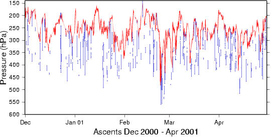
Ice-supersaturation layers appear mostly in a broad region below the tropopause, sometimes their tops reach into the stratosphere. This is shown in the following three plots. The red line marks the local thermal tropopause, the ice-supersaturation layers are marked by the vertical blue bars.
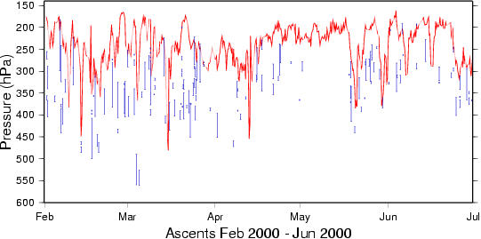
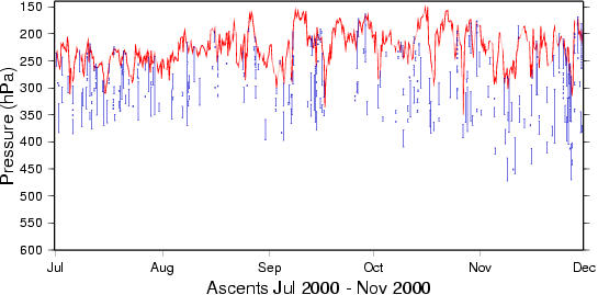
In the following plot, all pressure levels refer to the tropopause pressure. This shows how the ice-supersaturation layers are concentrated in a broad region below the tropopause.
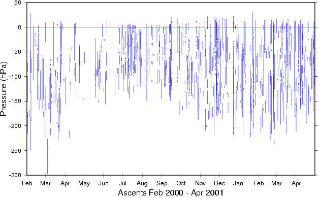
The depth of the upper tropospheric region that contains ice-supersaturation layers varies seasonally. It is relatively shallow in summer, and relatively deep in winter. The layer depths varies between 150 and 250 hPa. Ice-supersaturation layers extend often into the lowermost stratosphere, but not more than about 25 hPa in the Lindenberg data that we have analysed.