 |
Chemistry-Climate Model Validation Activity for SPARC (CCMVal) |
|
 |
Chemistry-Climate Model Validation Activity for SPARC (CCMVal) |
|
The Figures below are updates of
the figures published in Eyring, V., N. Butchart, D. W. Waugh,
H.
Akiyoshi, J. Austin,
S. Bekki,
G. E. Bodeker, B. A. Boville, C. Brühl, M. P. Chipperfield, E.
Cordero, M.
Dameris, M. Deushi, V. E. Fioletov, S. M. Frith, R. R. Garcia, A.
Gettelman, M.
A. Giorgetta, V. Grewe, L. Jourdain, D. E. Kinnison, E. Mancini, E.
Manzini, M.
Marchand, D. R. Marsh, T. Nagashima, P. A. Newman, J. E. Nielsen, S.
Pawson, G.
Pitari, D. A. Plummer, E. Rozanov, M. Schraner, T. G. Shepherd, K.
Shibata, R.
S. Stolarski, H. Struthers, W. Tian, and M. Yoshiki, Assessment of
temperature, trace species and ozone in chemistry-climate model
simulations of the recent past, J. Geophys. Res., 111,
D22308,
doi:10.1029/2006JD007327,
2006.
They include
new simulations stored at BADC.
Contact for questions: Veronika
Eyring
New model runs since
Eyring et al. 2006, 2007:
|
|
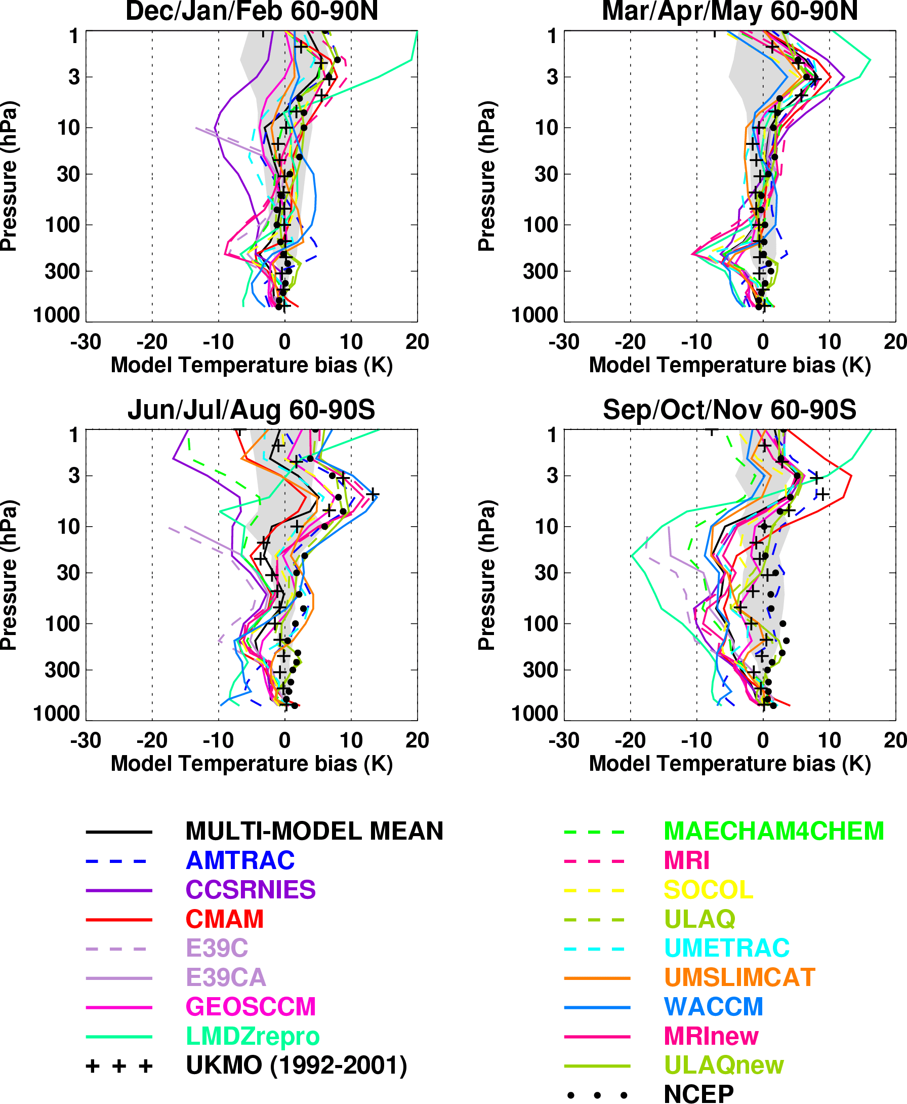 |
Figure 1. Climatological mean temperature |
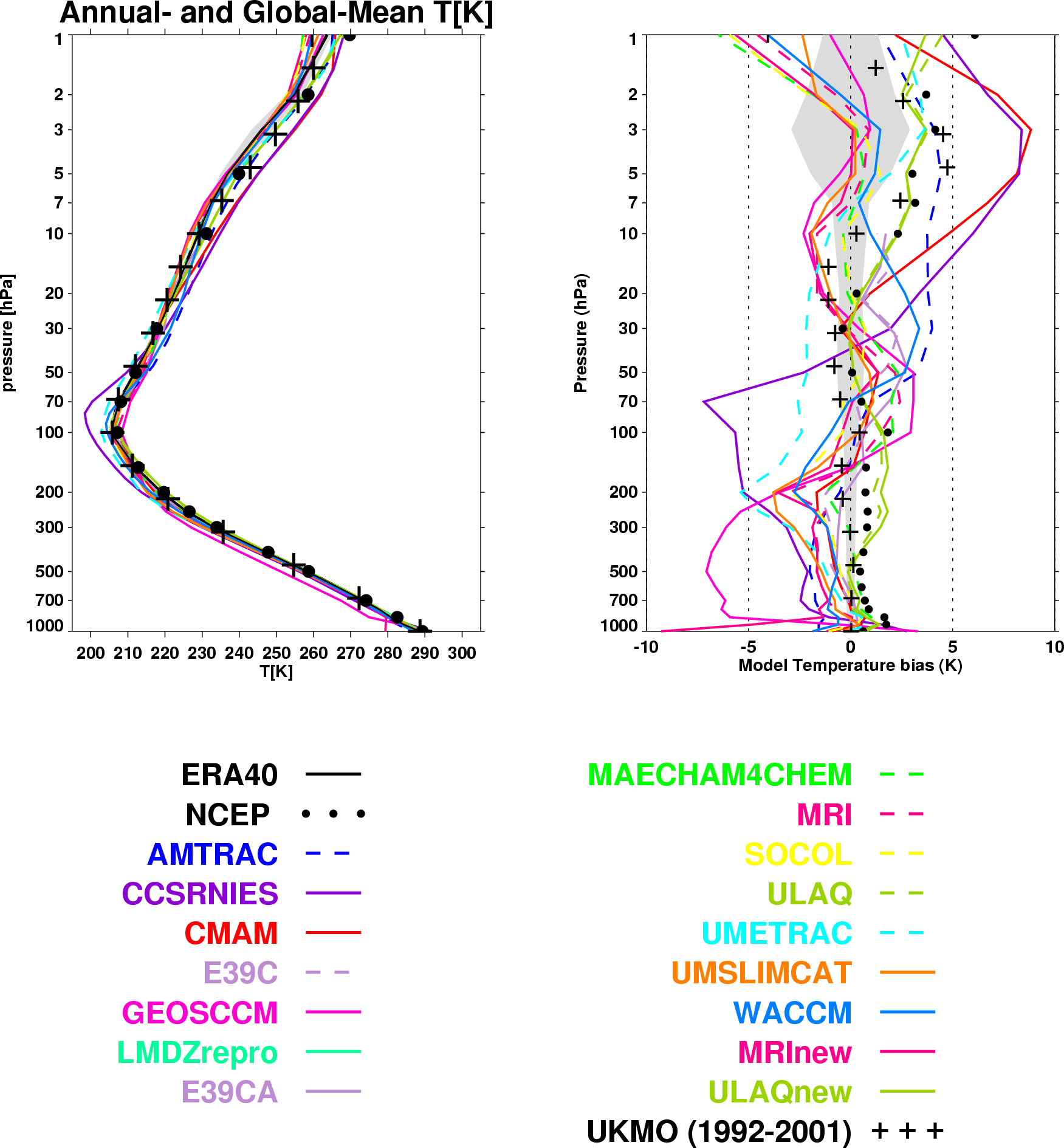 |
Figure 1b. Global annual mean temperatures |
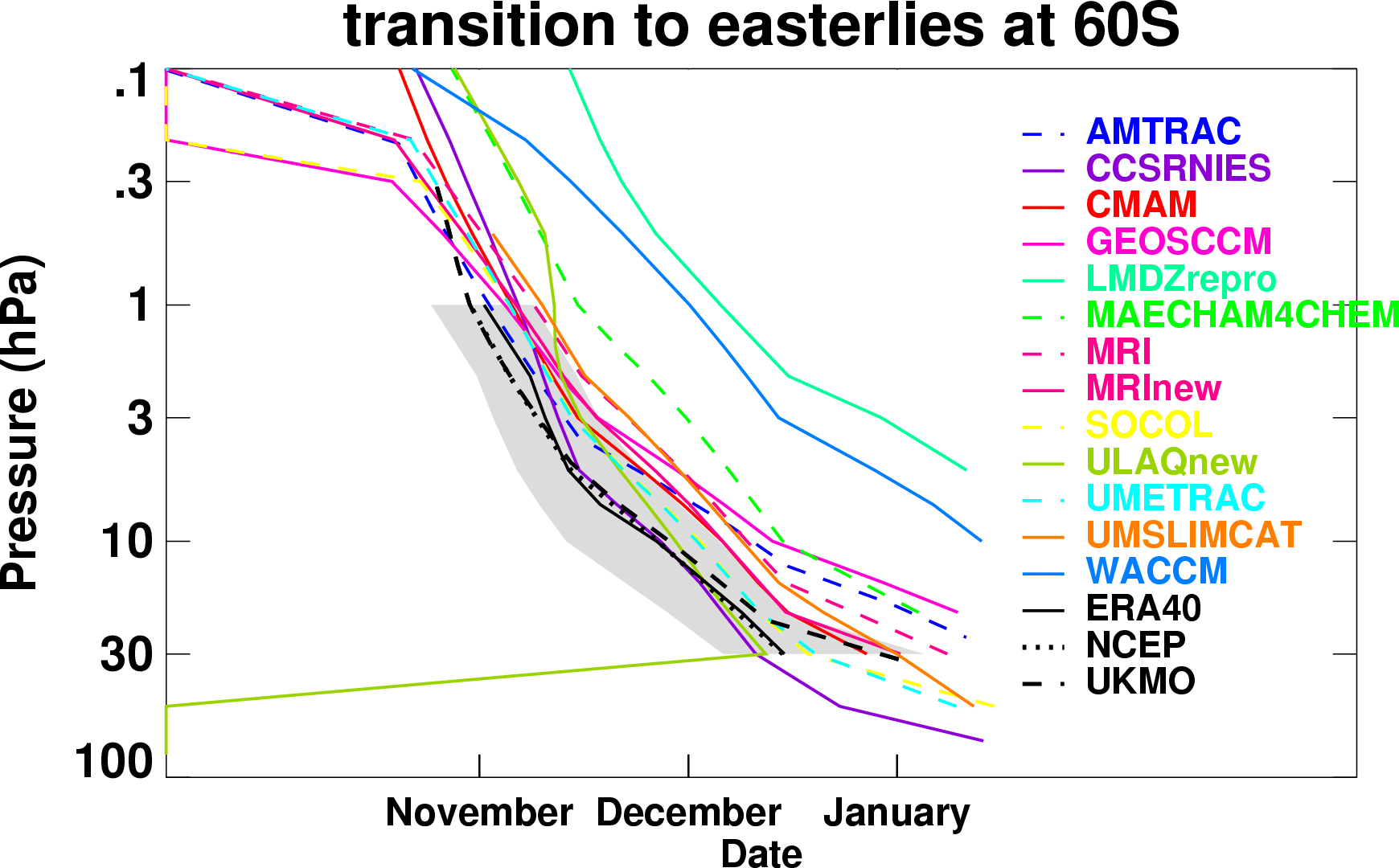 |
Figure 2. Descent of the zero zonal mean |
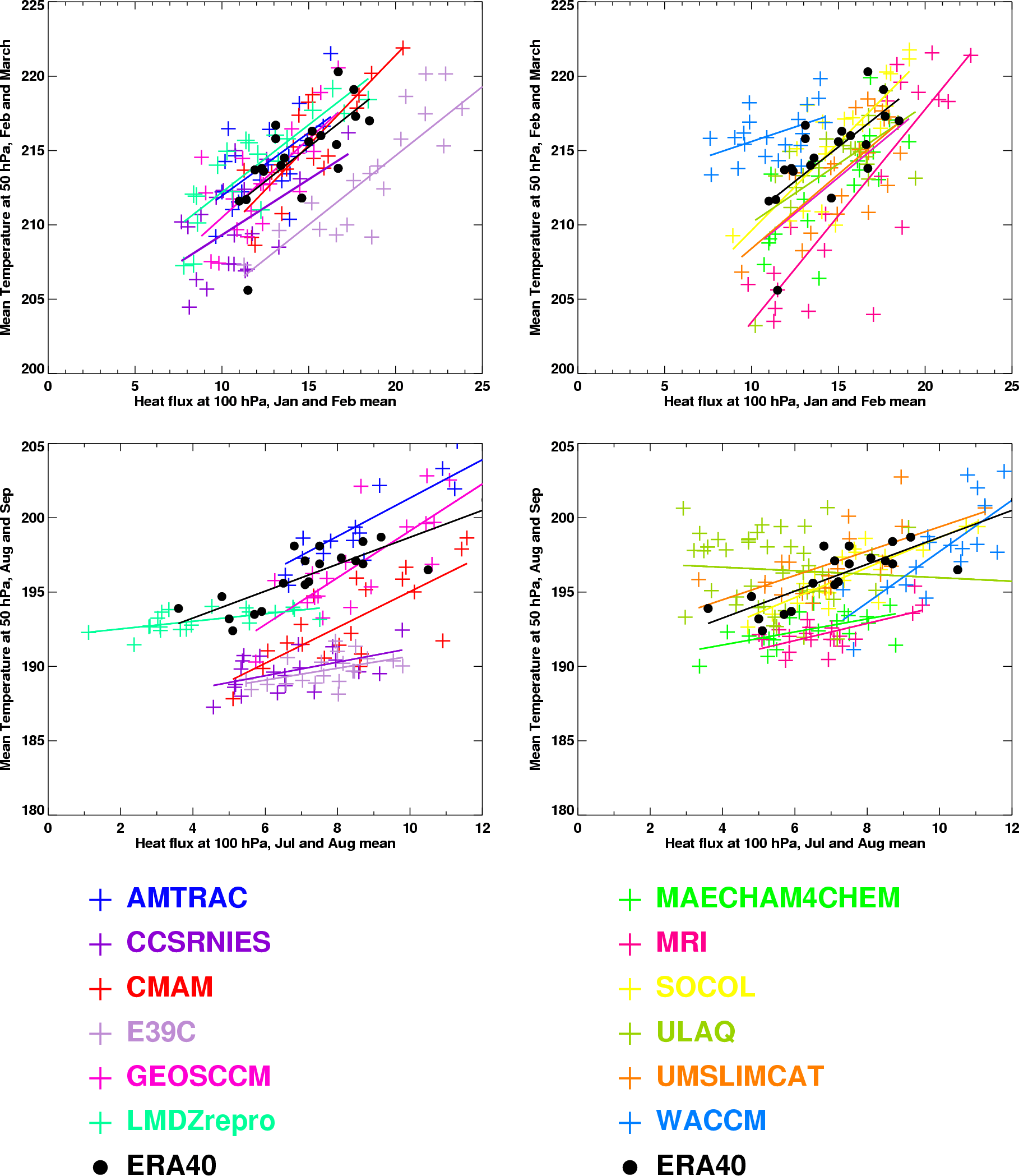 |
Figure 3. Upper
panels: Heat fluxes (v'T')
at
|
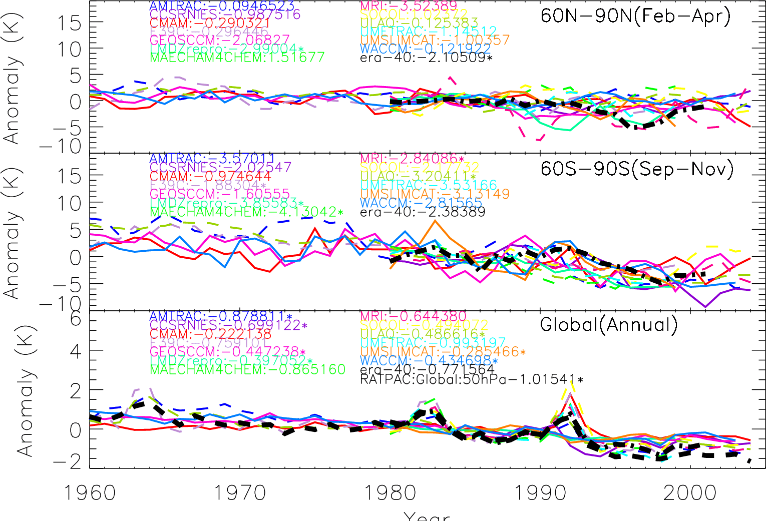 |
Figure 4. Modeled and observed time series of |
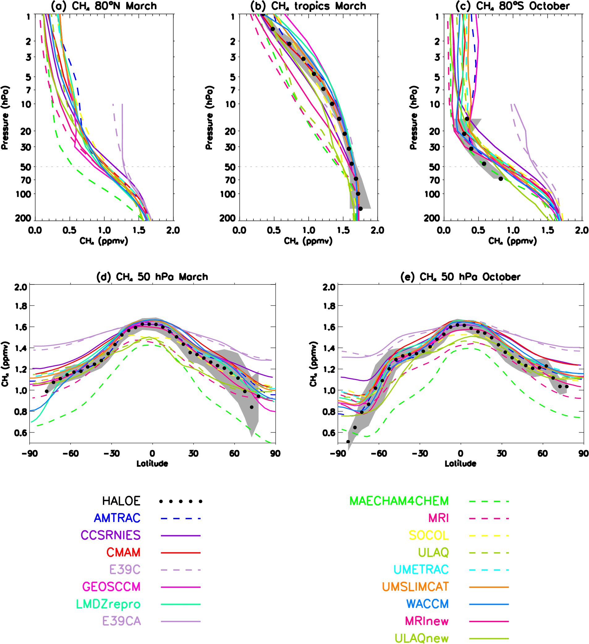 |
Figure 5. Climatological zonal-mean CH4 mixing |
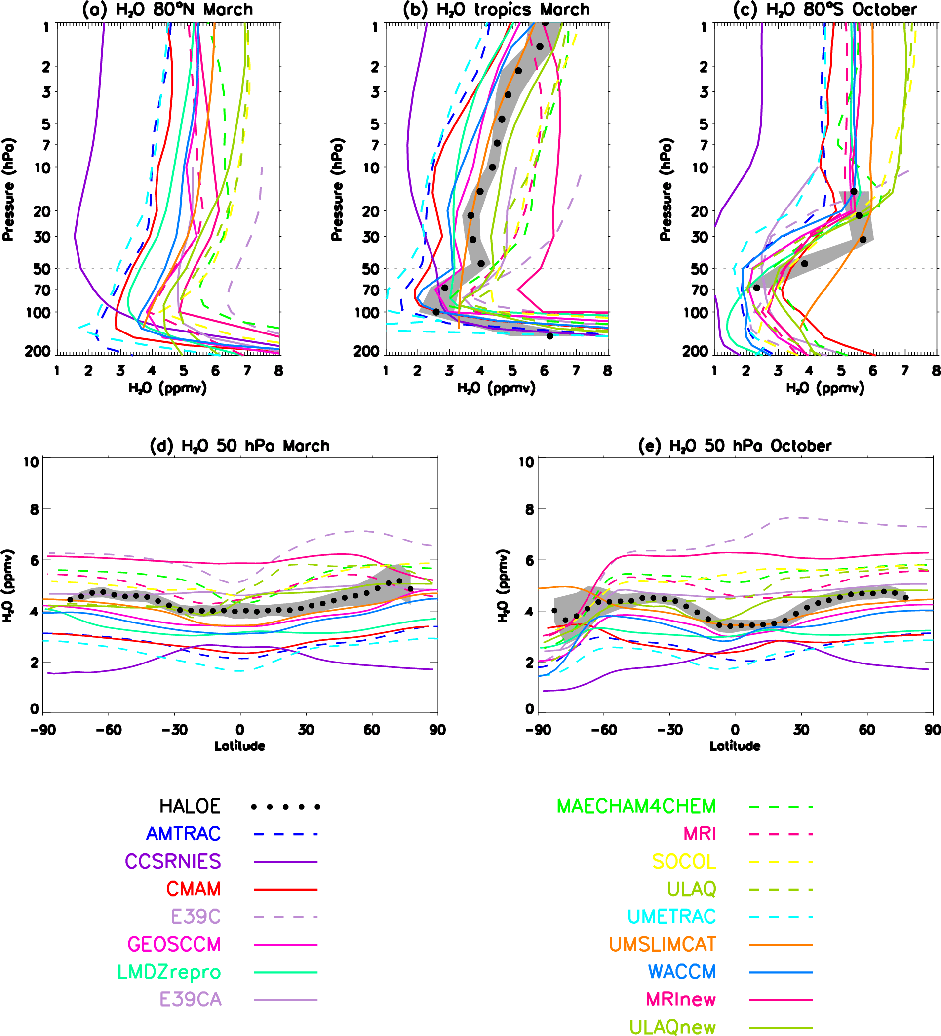 |
Figure 6. As in Figure 5, but for H2O
in ppmv. |
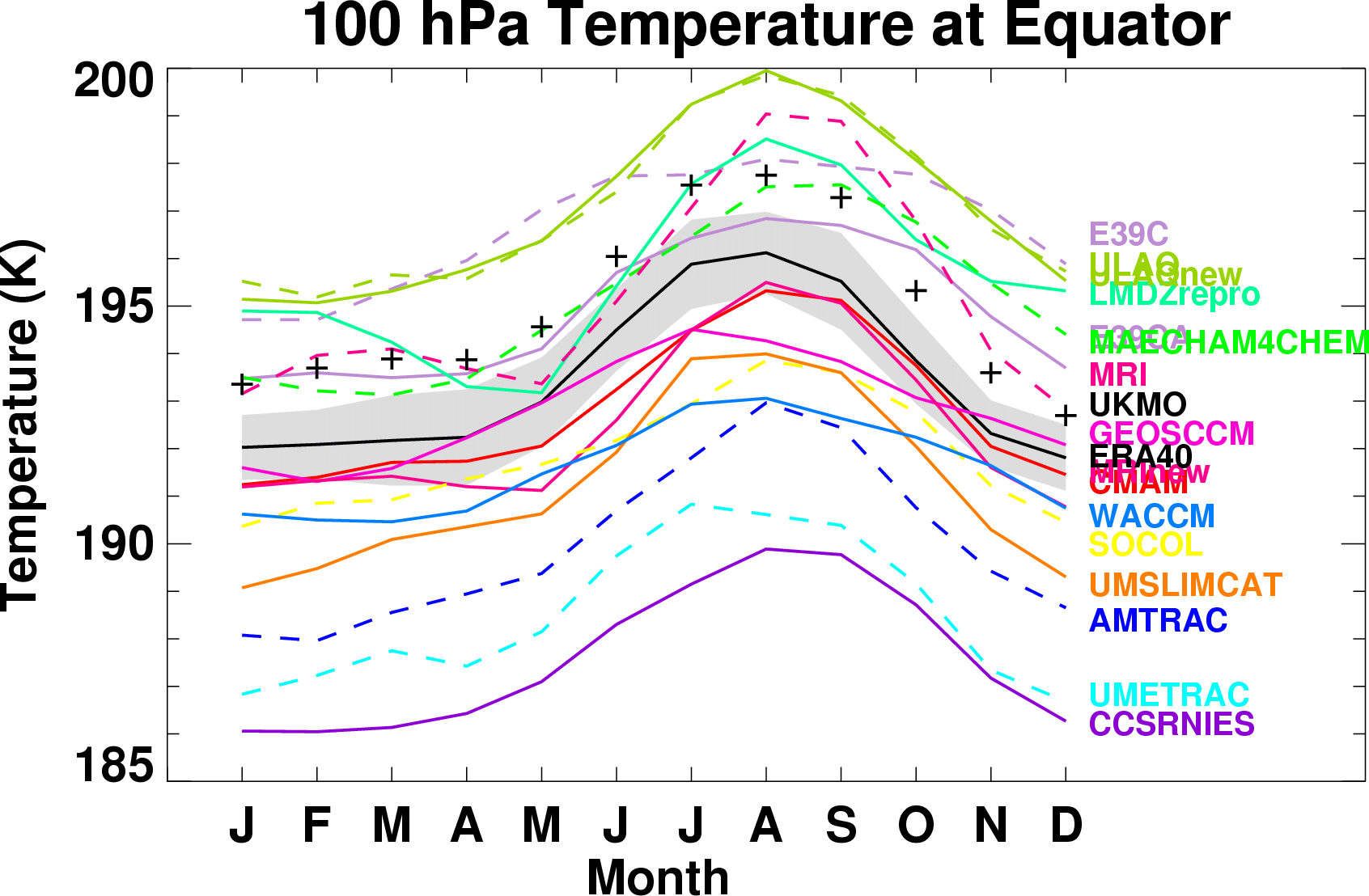 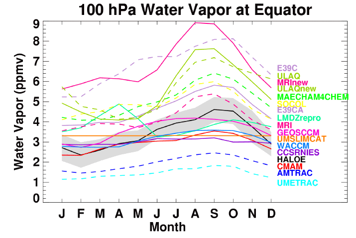 |
Figure 7. Seasonal variation of climatological means |
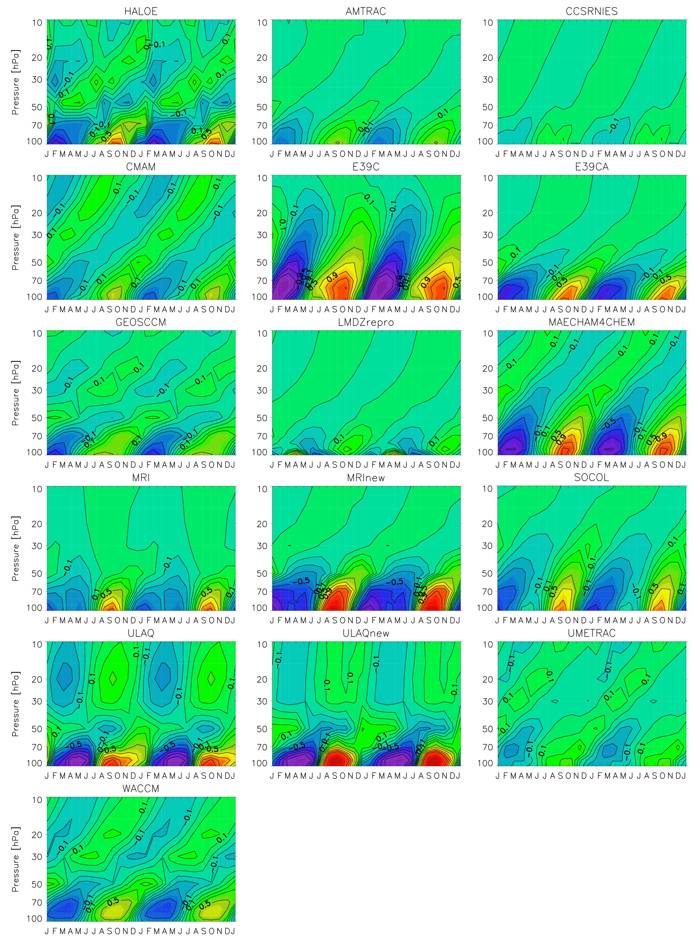 |
Figure 8. Time-height sections of water vapor |
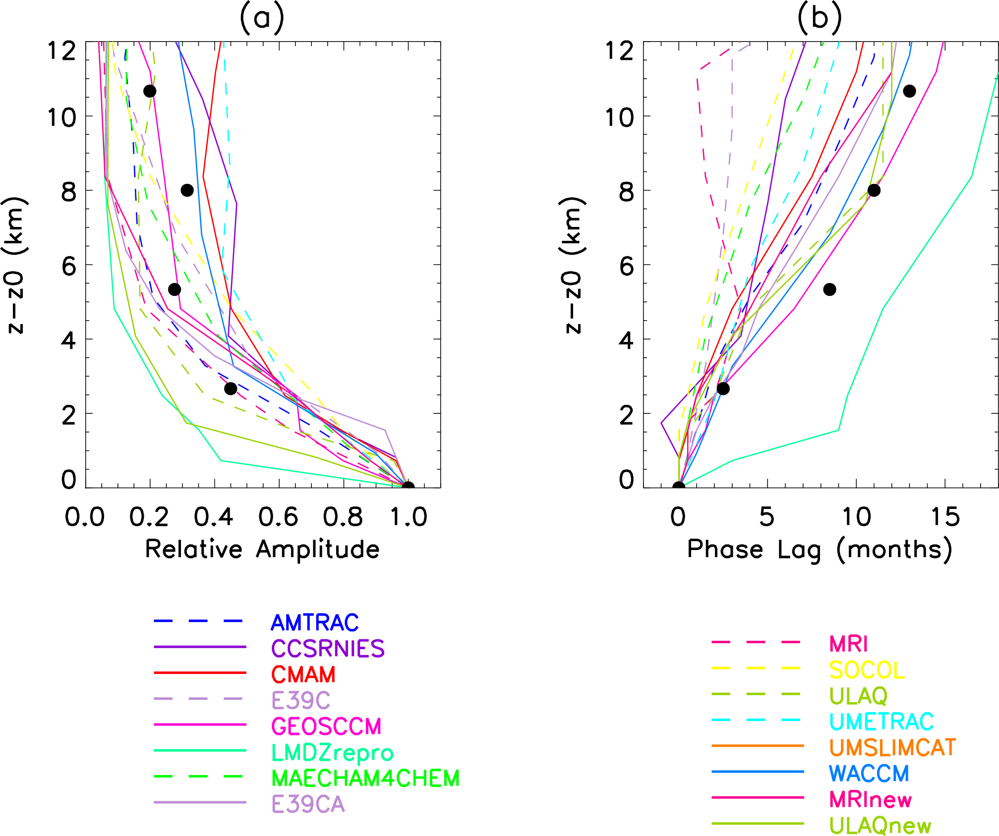 |
Figure
9.
Vertical variation of (a) amplitude and (b) phase lag of annual cycle of water vapor averaged between 10°S and 10°N. The amplitude is normalized to unity and phase lag is set to zero at the level (between 16 and 20 km) where the amplitude is maximum, which varies between the CCMs. The vertical axis in both plots is the distance from level of maximum amplitude. Solid circles are HALOE observations. |
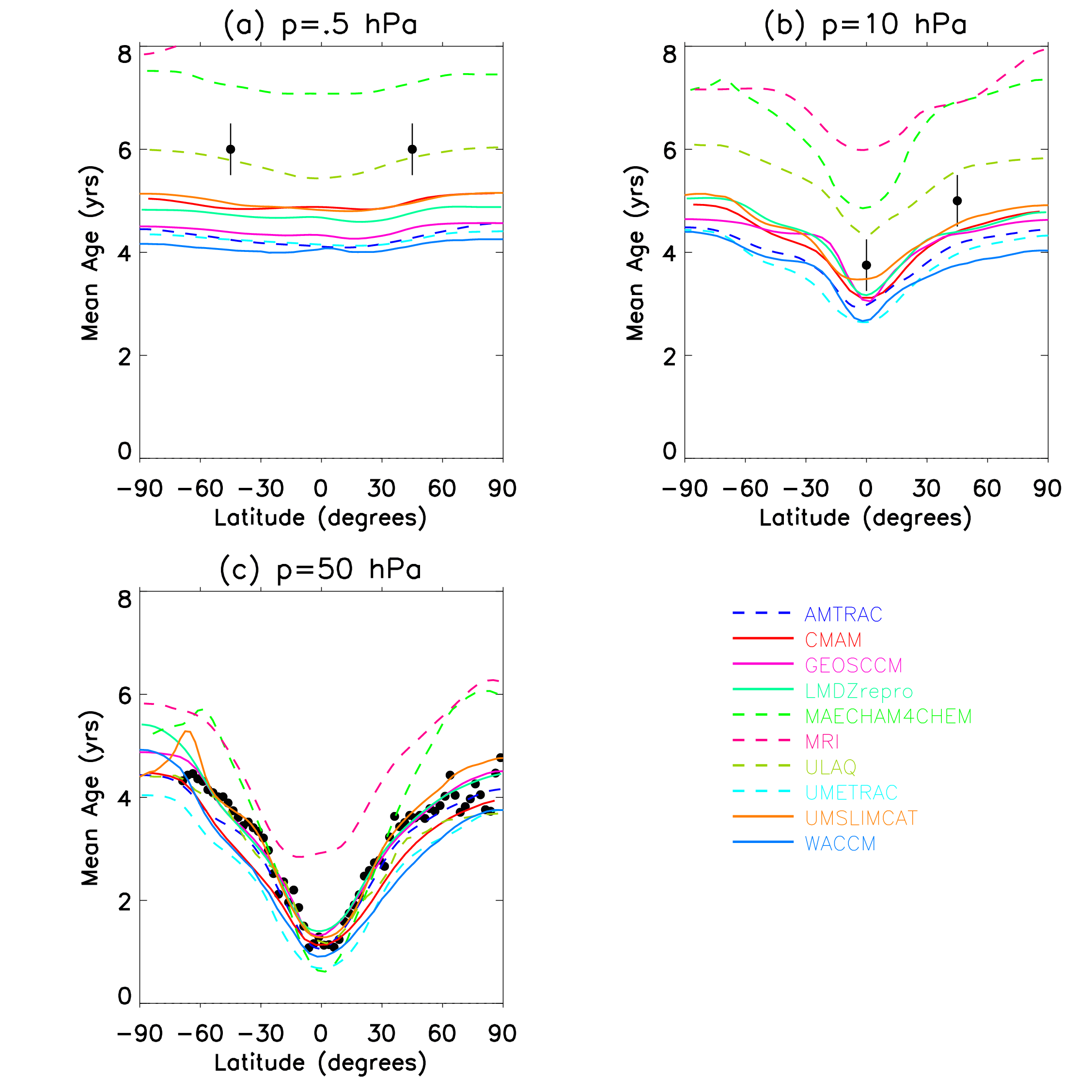 |
Figure 10. Mean age of air at (a) 0.5, (b) 10, |
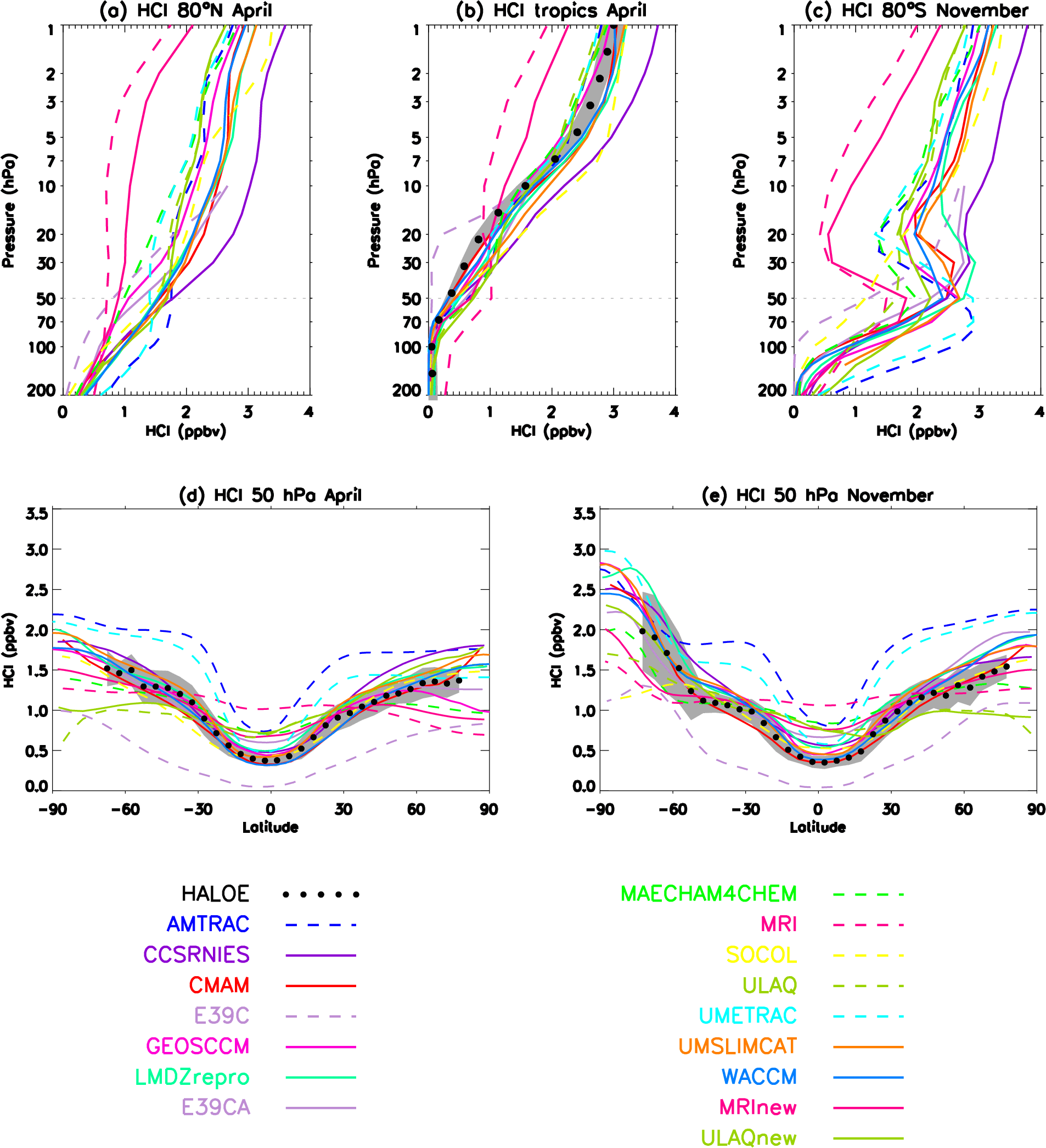 |
Figure
11. As
in
Figure 5, but for HCl in ppbv and vertical profiles are
shown at (a) 80°N in April (b) 0° in April and (c) 80°S in
November.
Lower panels show latitudinal profiles at 50 hPa in (d) April
and (e)
November. |
 |
Figure 12.
Left: Climatological mean vertical
profiles (1990 to 1999) at 80°S in
November for Cly in ppbv. Right: Time
series of October mean Antarctic Cly at
80°S from CCM model simulations. Estimates of Cly from
HALOE HCl
measurements in 1992 [Douglass et al.,
1995; Santee et al., 1996] and Aura
MLS HCl in 2005 [M. Santee, pers.
communication] are shown in addition. |
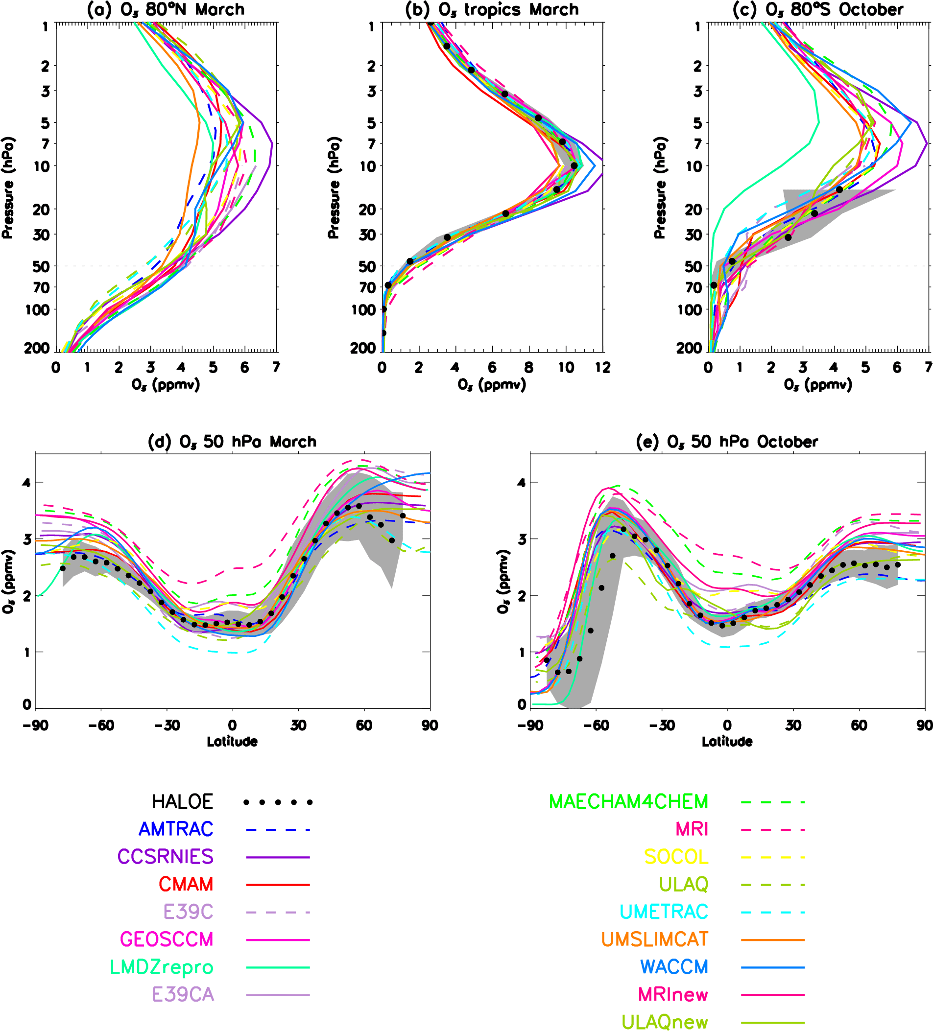 |
Figure 13. As in Figure 5, but for O3 in ppmv. |
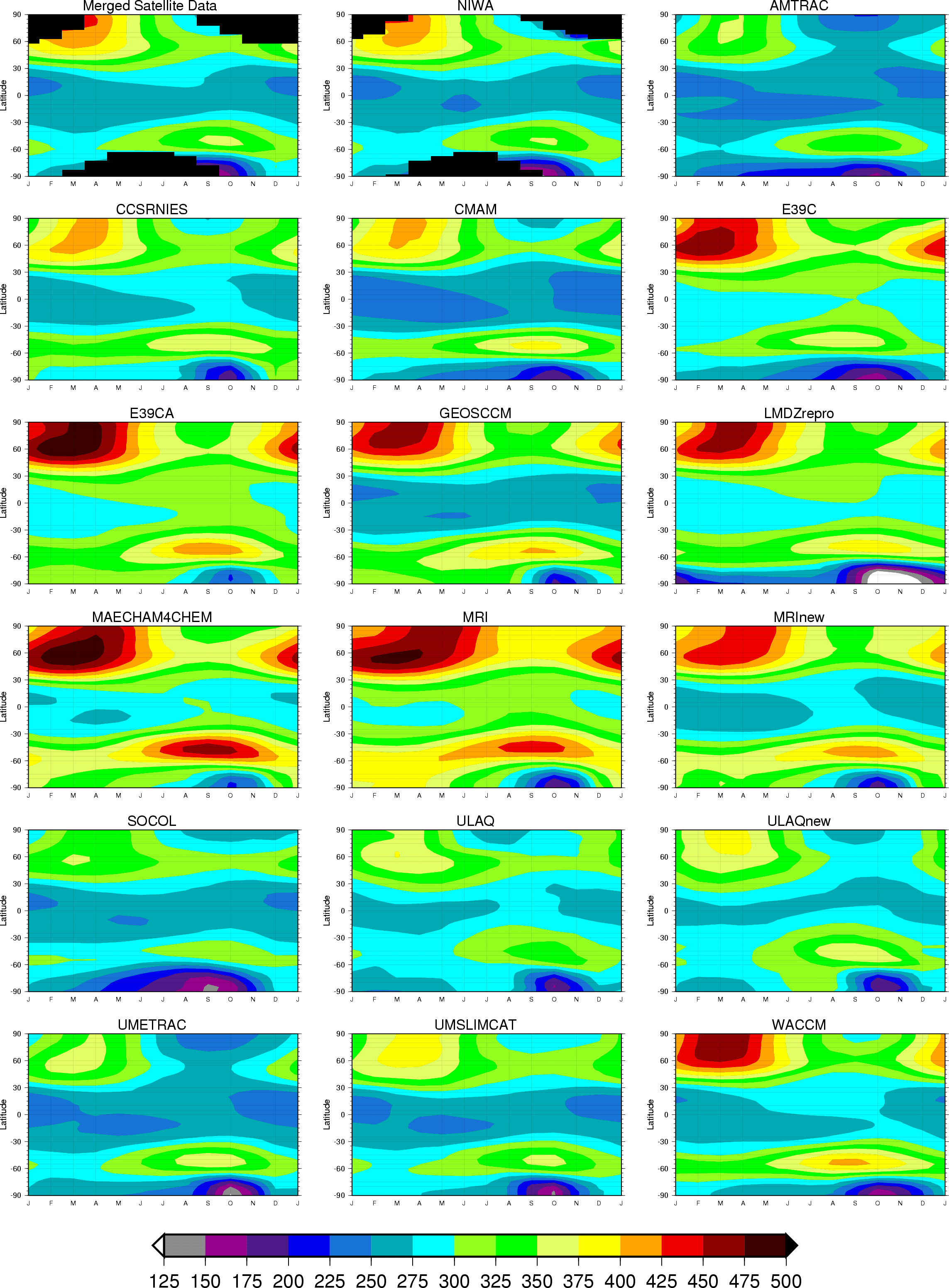 |
Figure 14. Modeled total column ozone climatologies (1980 to 1999) compared to merged satellite and NIWA assimilated data. |
|
Figure 15:
Left panels: (a) seasonal (February to April)
total column ozone anomalies for the Arctic (60oN-90oN),
(b) seasonal (September to November) total column ozone anomalies for
the
Antarctic (90oS-60oS), and (c) annual total
column ozone
anomalies sets for the whole globe (90oS-90oN)
from CCMs
and four observational data sets. The CCM results are shown with
colored lines
while the mean and range of the four observational data sets are shown
as a
thick black line and grey shaded area respectively. The anomalies are
calculated with the method described in Appendix A. The seasonal
anomaly time
series shown in panel (a) and (b) have been smoothed by applying a
1:2:1 filter
iteratively five times. The filter width is reduced to one at the ends
of the
time series. The annual global anomalies shown in panel (c) are
unsmoothed.
Right panels: detrended mean annual cycles for each model (1980 to
1989) and
the mean and range of the observations. |
| Last modified: 27 July 2007 | |
| by Veronika
Eyring |